Rotary Inverted Pendulum Control with Pole Placement

Fahmizal 1,*, Geonoky 2, Hari Maghfiroh 3

1,2 Department of Electrical Engineering and Informatics, Vocational College, Universitas Gadjah Mada, Indonesia

3 Department of Electrical Engineering, Universitas Sebelas Maret, Indonesia

Email: 1 fahmizal@ugm.ac.id, 2 geonoky@gmail.com, 3 hari.maghfiroh@gmail.com 

*Corresponding Author

Abstract—This research focuses on the analysis of inverted pendulums, specifically the rotary inverted pendulum, which is a multivariable and highly unstable dynamic system. Inverted pendulums are commonly employed in studying modern control and control system designs due to their challenges related to nonlinearity, complexity, and inertia. The rotary inverted pendulum, in particular, is investigated in this paper, with a primary emphasis on utilizing state feedback adjusted by pole placement. The objective is to guide the pendulum along a circular path, eliminating the challenges associated with the traditional transversal path. The careful selection of design parameters is crucial to ensure that the pendulum reaches a stable equilibrium point. The study underscores the importance of addressing the specific area where the pendulum is expected to reach this point of agreement.

Keywords—Inverted Pendulum; System Modeling; Pole Placement

1. Introduction

The control system means commanding, regulating, and directing both physically and dynamically. Hence, the design of a control system depends on what elements are to be regulated, commanded, or directed according to the designer. One example is an inverted pendulum. Inverted pendulums have been widely used in linear and nonlinear control systems with applications to less active mechanical systems involving nonlinear dynamics, robotics testing, and vehicles. A wide variety of resources have been produced to support teaching, emphasizing complex processes that enable us to better understand how to handle control system design. For example, such as the Rotary Inverted Pendulum [1], [2].

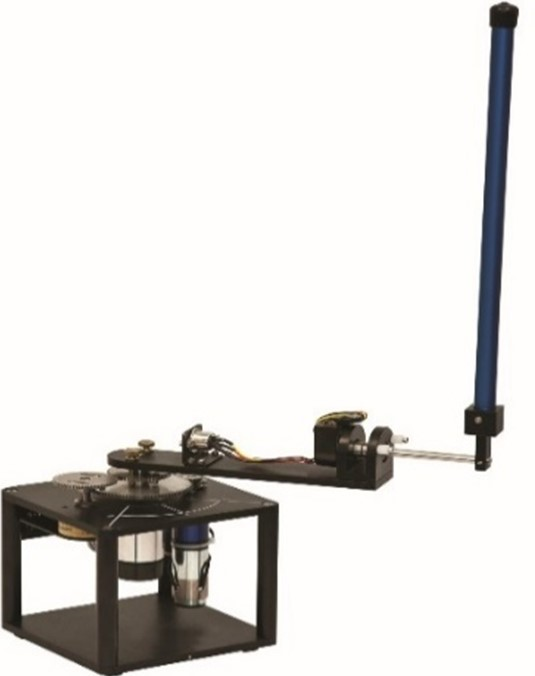
The Rotary Inverted Pendulum is a system that has two degrees of freedom (DOF), namely clockwise and anti-clockwise. This system is integrated with three elements: a motor and two rods called the arm and pendulum. The rotary inverted pendulum is shown in Fig. 1, the way the system works is how to balance the pendulum connected to the arm. The arm functions as a link between the pendulum and the DC motor. The function of the DC motor here is to provide rotation which allows the pendulum to carry out balancing movements. An inverted pendulum has characteristics of nonlinear, unstable, under-actuated, multivariable, and fast dynamic [3], [4].

The rotary inverted pendulum involves physical modeling concepts and tools for validating regulators in automatic control [5]. A pendulum that rotates freely in the vertical plane is assembled from the other end of the arm. The rotary inverted pendulum is a compact and simple system that shows control problems can be managed. Some examples of the inverted pendulum in daily life applications are missile launchers [6], balancing robots [7], and humanoid robots [8]. This problem, being physical, allows us to construct nonlinear equations of dynamic behavior based on Newton's laws [9].

1. Rotary inverted pendulum

As observed in Lundberg and Barton [10], the approach that has been used considers a linear model, where the process is simplified to treat it as if it were a linear system. The rotary inverted pendulum is a process that allows teaching the use of state space modeling techniques, linearization, regulatory controller design, and sensitivity analysis. This is a classic problem that allows simple schemes such as PID control to be tested up to complex control schemes, such as SMC control. Attempts have also been made to achieve global stability in these processes, separating them into systems where a swing-up is performed to move the pendulum away from a stable equilibrium position, and then switching to another controller tasked with keeping the pendulum stable at an unstable equilibrium point.

The rest of the paper is as follows: Section II discusses the materials and method which include the overview of modeling of the rotary inverted pendulum and the proposed method. The results and discussion are presented in Section III. Finally, the conclusion of this research is resumed in Section IV.

2. Materials and Method

1. Materials

1. Modeling of rotary inverted pendulum

A schematic image of a rotary inverted pendulum (RIP) with several parameters is shown in Fig. 2. The Rotary Inverted Pendulum modeling is considered using a system based on the Quanser inverted rotary pendulum [11]. In this system, the dynamic equation is obtained as (1) to (3).

2. Schematic rotary inverted pendulum (RIP)

As seen in Fig. 2, x1 is the arm angle while x2 is the pendulum angle. The parameter values are listed in Table 1. To define two additional variables x3=x1 and x4=x2, equations (1)-(3) can be expressed as a first-order nonlinear system in equations (4)-(5) as follows:

1. Parameter values of rotary inverted pendulum model

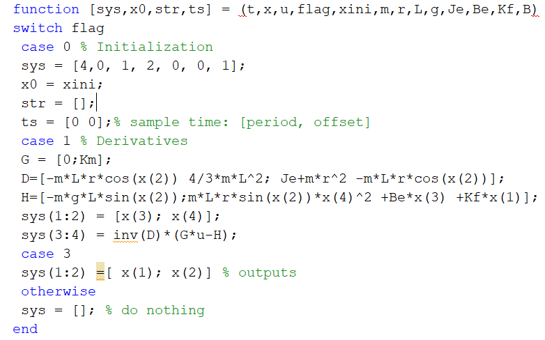
With the output y=[x1 x2]T is a linear expression containing both angles, namely the arm and the pendulum. If we define X=[x1 x2 x3 x4]T with equation (4), then we obtain the standard representation of equation (9). According to K. Munoz and Poblete [1] with this representation in state variables (9) a Simulink / MATLAB function model is created (Fig. 3). In this model the parameters are shown in Table 1 and xini is defined as a vector containing the initial conditions of the arm angle, pendulum, and respective angular velocity.

3. MATLAB s-function for RIP

From equations (10) and (11) in equilibrium x3=0 and x4=0. Where it can be concluded that the manipulated variable must be zero and there are infinite solutions for the pendulum angle in equilibrium, which corresponds to x2 = nπ where n is an integer. If n is even, then the equilibrium position for the pendulum is up (inverted pendulum) and if n is odd, the equilibrium position for the pendulum is down (normal pendulum). Likewise, x2=0 is the balance position for the pendulum in an inverted state.

2. Linearization

The analysis techniques that will be used only apply to linear systems. Because the goal of the control system is to keep the pendulum upright, the equation that has been obtained must be linearized. Linearization of this equilibrium state system can be achieved by carrying out a first-order Taylor series expansion for the functions f(x,u) and h(x,u), so that the equation (12) is obtained. Where Ψ(x,u) represents the component of the order greater than 1. Note that for points very close to equilibrium it is true that Ψ(x,u)≈0.

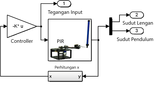
Matrices A, B, C, and D are obtained as equations (13), (14), (15), and (16), respectively. When evaluated at the equilibrium point it is calculated by equations (10) and (11). Fig. 4 shows the Simulink model, where the feedback control system is configured.

4. Close loop control model of rotary inverted pendulum in simulink, Tegangan input (Input voltage), Sudut lengan (Arm Angle), Sudut pendulum (Pendulum angle), Perhitungan x (x Calculations)

5. MATLAB code for RIP linearization

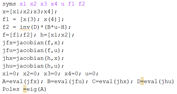
Fig. 5 makes it possible to obtain by symbolic algebra the values of these matrices. It should be noted that there is no relationship that depends on the value of x1 at equilibrium, where the matrix generated in equations (17) to (19) is identical for each arm angle that we want to operate, where with these equations we can perform reference tracking for the arm by creating change of coordinates to refer to the new angles of the arm to the desired position.

Eigenvalues of matrix A, obtained with the MATLAB function eig(A). The system values obtained are -9.4328, 8.9784, -0.3069 + 3.3250h and -0.3069 - 3.3250h. One of the poles is positive, which indicates that the system is unstable at this equilibrium point.

In controller design, system stability can be verified from the location of the system poles in the complex plane. The system is said to be unstable if one of the poles is on the right side of the complex plane. However, on the contrary, the system is said to be stable if all the poles are located on the left side of the complex plane. For an unstable system, a control method is needed that can bring all poles to the left of the imaginary axis to become a stable system [12].

The control system must be able to be checked whether the system can be controlled in full condition or not. If the A and B matrices of the state space model can be controlled, then the system can be controlled by placing the poles in a full state. The resulting system is fully controllable at the balance point, namely with the controllability equation M=[B AB A2B A3B] equal to the number of states in the system (rank(M)=4) [13]. This problem does not require a state observer because the first two components of the state vector are the arm and pendulum angles, and the last two components of the state vector can be reconstructed by deriving these angles.

2. Method

One type of state feedback control is pole placement. Pole placement control is a way to place poles arbitrarily according to the characteristics we want. However, there are still criteria that we must fulfill before starting to use pole placement. The first criterion is that all the state variables that we define must have known values. If one of the states is not known, then an observer is used to estimate it.

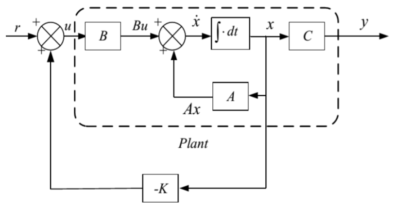
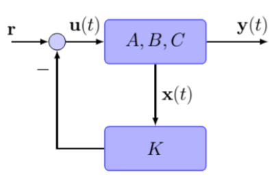
Pole placement control aims to stabilize an unstable system or to improve its performance in terms of stability so that transients turn off very quickly. Fig. 6 illustrates the full state feedback block diagram in the state space model and is more simply presented in Fig. 7.

6. Full state feedback detailed block diagram

7. Full state feedback simplified block diagram

It is assumed that the desired closed-loop poles are set at s=p1, s=p2, s=p3, ..., s=pn by choosing the right gain matrix to represent the feedback. It is easy to set the closed-loop poles of the system at the desired location in the complex field when the system is completely under control. For the selection of desired closed-loop poles in complex fields, there is a compromise that needs to be made between the response to the speed error and the responsiveness to interference and measurement noise. If there is an increase in the response speed of the displayed error, then there will be an increase in the harmful effects of the interference and measurement noise displayed.

A linear dynamic system in the form of a state space is shown in Equation (20) and Equation (21), where D is zero [14], [15]. To improve system stability, the full state feedback control law is considered proportional to the state.

The Lyapunov function is defined as:

Derivative in time V(x) as:

And combined using equation (23) then:

The condition for (26) always be negative if the values of K are such that the eigenvalues of A-BK all have a negative real part, and this Ψ(x) is contained in the small neighborhood for compliance with (26). If equation (26) is satisfied, then it can be ensured, according to Lyapunov's theorem, that the system fed back to the controller (22) will be stable.

The closed-loop poles are located using the place routine in the MATLAB control toolbox. This value for the desired closed-loop pole is set considering that the expected time for the pendulum and arm to stabilize is 4 seconds. Note that the controller design influences the range of x values satisfying equation (12). It was considered to design two controllers using the pole placement technique. The first controller, named C1, is designed such that the poles of the closed-loop controller are located at {-1, -5, -1-3i, -1+3i} and the second controller, called C2, is designed such that the closed-loop poles are located at {-5, -4.1, -5-3i, -5+3i}, poles are selected to meet the stated requirements.

The most relevant variable in this process is the angle of the pendulum, and the goal is for the pendulum to remain in an upright position. Although, interestingly, the arm angle reaches the reference, it has been considered a performance function that only considers the evolution of the pendulum angle. To evaluate the performance of the system, the maximum absolute value achieved by the pendulum angle is considered as a cost function (27).

This value is chosen because if it reaches the normal stable position (pendulum hanging down) or MP ≥ π, at any time in the specified time interval between start time zero and end time(tf), the system is then considered unable to hold the pendulum in reverse. The value of tf is considered large enough to ensure that the system has been able to reach its equilibrium condition because the establishment time is determined in 4 s, the value for this time is set in tf = 5 s.

3. Results and Discussion

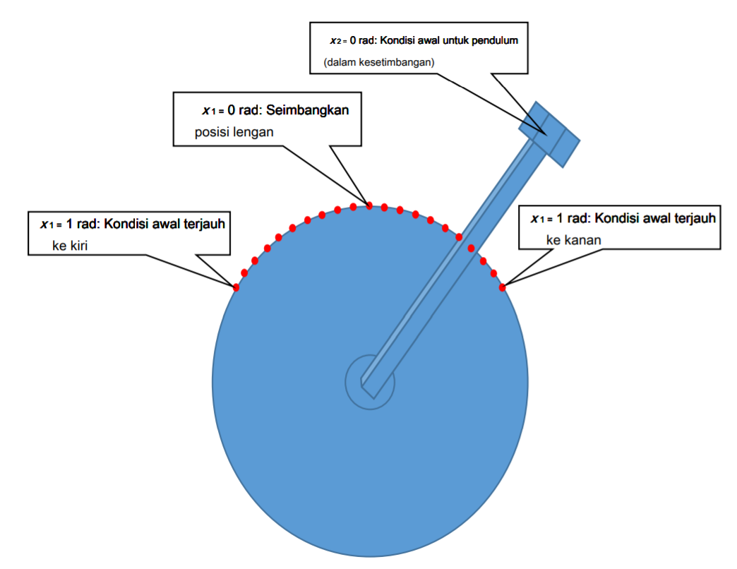
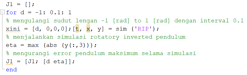
Two experiments are considered in which the performance of the closed-loop system is compared with both controllers (C1 and C2). The first experiment aims to analyze how the starting angle of the arm affects the system performance. For this reason, the RIP is initialized from various arm angles, as shown in Fig. 8. As can be seen, the pendulum starts from an inverted equilibrium position with an initial angle d for the arm, zero for the pendulum, i.e., in a vertical position and stops with zero velocity for the arm and pendulum (x1=d, x2=0, x3=0, and x4=0). It runs repeatedly with variable d (see code shown in Fig. 9).

In each iteration the instruction [t, x, y] = sim('RIP') is executed, calling the model into RIP.slx (Fig. 4) and running it for 5 seconds with the initial condition xini = [d, 0, 0, 0]. In this way, 21 simulations are carried out, starting from the arm angle, from -1 [rad] to +1 [rad] separated every 0.1 radians, that is, sweeps are made from about 57 degrees to the left and right of the equilibrium point. The variables that return the instruction ([t,x,y] = sim('RIP')), correspond to a matrix where each column contains the signal values indicated at the output gates listed in Fig. 4.

8. Top view of the rotary inverted pendulum, red dot shows the simulation's initial position

9. First simulation coding

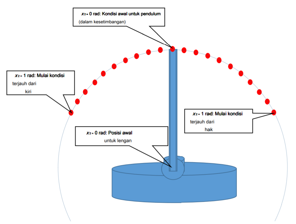
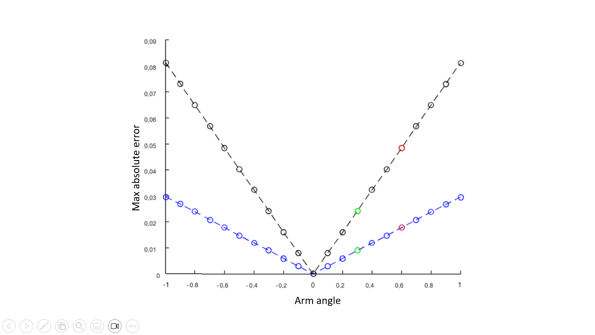
The second experiment starts from the system for different pendulum angles as shown in Fig. 10. In this case the initial pendulum angle ranges from -1 rad to +1 rad, every 0.1 radians, but with positions initial xini = [0, d, 0, 0]. It is assumed that the remaining initial conditions are zero, that is, the system always starts with the arm in an angular position of zero radians, and the arm and pendulum are stopped at the beginning (x1=0, x2=d, x3=0, and x4=0). After carrying out the simulation, the first experimental results were obtained which are presented in Fig. 11 and Fig. 12. In Fig. 11, each circle represents the maximum absolute error calculated by (27) for the initial conditions shown on the ordinate axis.

10. Lateral pendulum, red dot shows the simulation's initial position

11. Performance of a closed-loop system with controllers C1 (in blue) and C2 (black) under different initial conditions of arm angle, keeping the remaining variables at the equilibrium point

From the obtained simulation results as the initial angle increases, the maximum absolute error presented by the pendulum angular response will also increase. Fig. 12 shows that the growth rate obtained with controller C2 is greater than that obtained with controller C1. From the results shown in Fig. 11 the circles colored red and green, indicate the maximum absolute angular errors reached in the pendulum for two specific cases: when the simulation starts with arm angles of 0.3 [rad] and 0.5 [rad], respectively.

12. Response of a closed-loop system with controllers C1 (in blue) and C2 (black) for initial conditions of arms 0.3 [rad] (left) and 0.6 [rad] on the right, keeping the remaining variables within the balance point

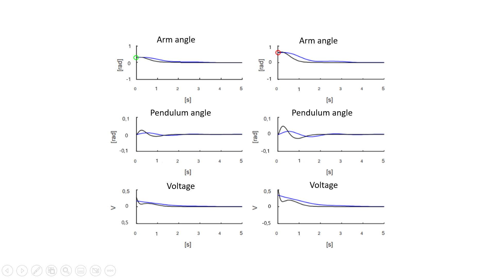
Fig. 12 shows the reaction curve of the angular response of the arm, pendulum, and voltage applied to the motor when the initial conditions are the initial conditions marked in the previous figure: 0.3 [rad] on the left and 0.5 [rad] on the right. If you look at the graph on the left side, the first one marks 0.3 [rad] for the arm (see green circle), and the middle one marks 0 [rad] as the initial condition for the pendulum. The middle graph shows that the maximum error achieved by the arm is 0.03 rad with controller C1 (in black) and a much less high value with controller C2 (in blue).

In the resulting graphic image, it can be observed that the stabilization times achieved with both controllers are the same and meet the design requirements. In the graph on the right, the responses obtained with both controllers when the initial arm condition is 0.5[rad] are observed. It is observed that this maximum pendulum error is larger with controller C1 (in black) than with controller C2 (in blue).

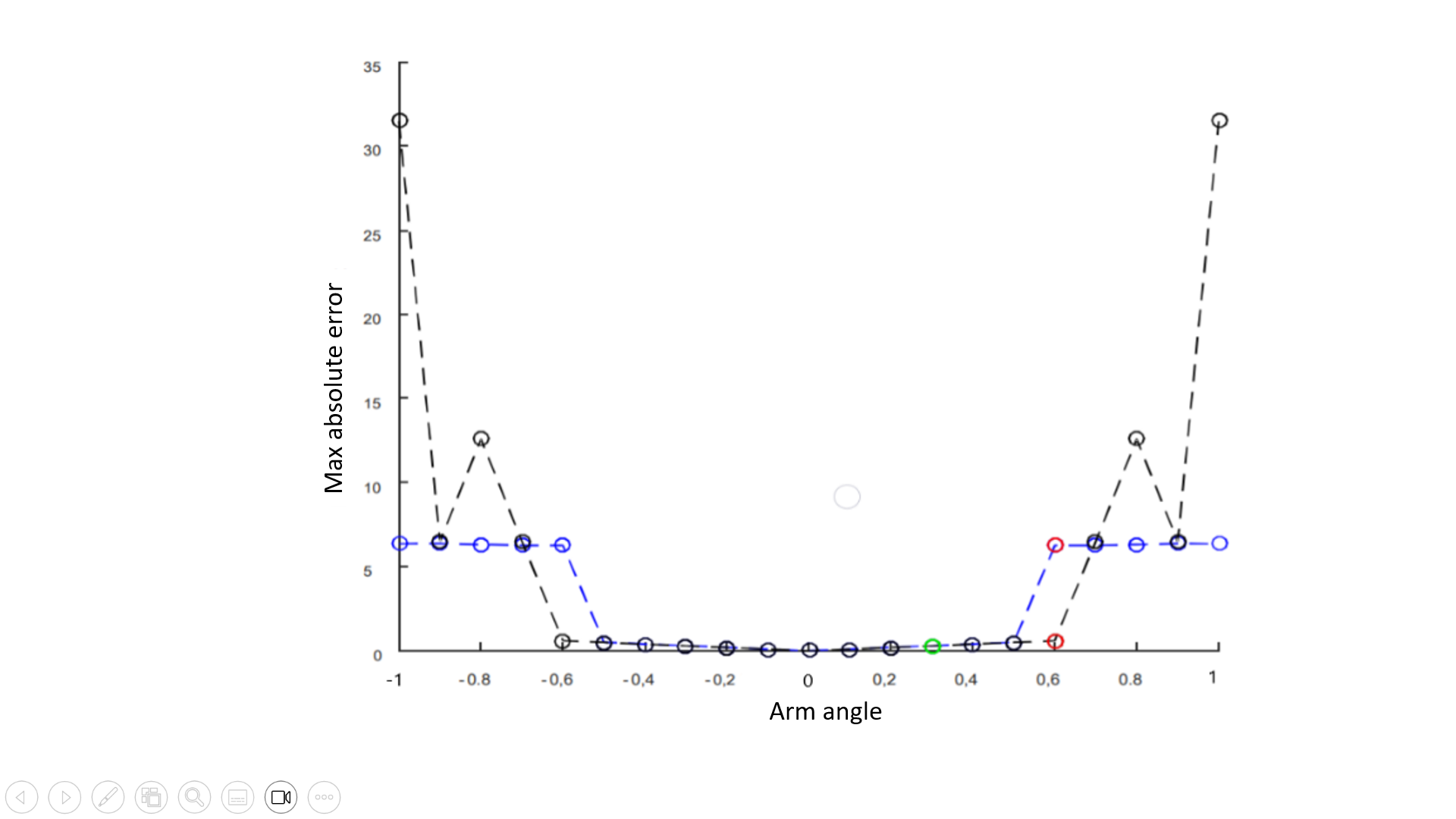
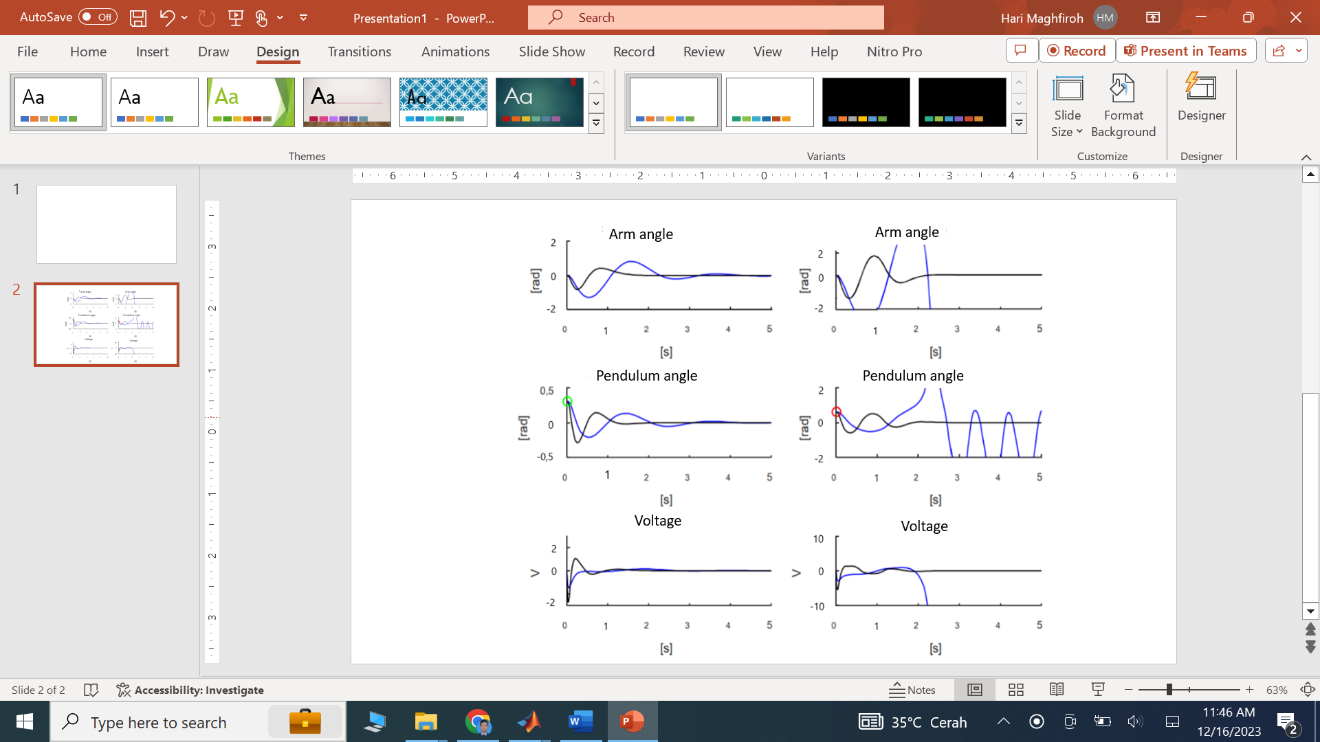
The results of the second experiment are presented in Fig. 13 and Fig. 14. As in Fig. 11, each circle represents the maximum absolute error calculated by (27) during the 5 s simulation. The initial conditions are shown on the horizontal axis, which this time corresponds to the initial angle of the pendulum because the initial condition of the arm is zero and the angular velocity of the arm and pendulum is zero. It is observed that as the initial angle increases, the maximum absolute error of the angular path of the pendulum also increases and that within ± 0.5 [rad] this index starts to take values greater than 3 [rad] for controller C1 (in blue), with controller C2 (black) something similar happens but for higher values ±0.6[rad]. When this angle reaches a value greater than 3[rad] it means that the pendulum falls from an unstable equilibrium position, so the results obtained with the maximum absolute error of the pendulum greater than 3[rad] should be rejected, considering that the controller cannot meet the requirements which are determined.

In Fig. 13, like the previous scenario, red and green circles are utilized to represent the maximum absolute errors in pendulum angles during simulations starting with initial pendulum angles of 0.3 [rad] and 0.5 [rad]. Moving on to Fig. 14, the left side illustrates response curves for both controllers (C1 in blue and C2 in black) concerning the arm angle, pendulum angle, and the motor voltage. These responses are observed when the simulation begins with an initial condition of 0.3 [rad] for the pendulum (depicted by the green circle). Specifically, the initial conditions include 0 [rad] for the arm, zero initial velocity for both the arm and pendulum. On the right side of Fig. 14, a similar analysis is presented, but this time the initial condition of the arm is set at 0.5 [rad] (indicated by the red circle in the top-right graph). The initial angle of the pendulum is maintained at zero (middle-right graph), along with zero initial angular velocity for both the arm and the pendulum. This comprehensive examination provides insights into the system's behavior under different initial conditions and the corresponding controller responses.

13. Performance of a closed-loop system with controllers C1 (in blue) and C2 (black) under different initial conditions of pendulum angle, keeping the remaining variables at the equilibrium point

14. Response of a closed-loop system with controllers C1 (in blue) and C2 (black) to the initial pendulum condition of 0.3 [rad] (left) and 0.6 [rad] to the right, keeping the remaining variables at the equilibrium point

4. Conclusion

This research aimed to implement a state feedback controller using the pole placement method for designing a control system tailored to a rotary inverted pendulum. The pole placement control technique facilitates the strategic placement of poles to achieve desired system characteristics. The step-by-step elucidation presented in this study guides the resolution of the controller design challenge through state feedback, ensuring the rotary inverted pendulum attains stability at an equilibrium point, despite its inherent instability. The process involves nonlinear representation in state space, balance point computation, linearization, controller design, and performance function definition. Notably, the nonlinear dynamics of the rotary inverted pendulum introduce a complexity wherein the feedback system exhibits variable behavior in response to diverse initial conditions, potentially causing destabilization. This exploration enhances our understanding of control strategies for inherently unstable systems, paving the way for more robust and adaptive control methodologies.

References

1. C. Muñoz-Poblete, "Pole placement controller applied to a Rotary Inverted Pendulum System. A didactic view," 2018 IEEE International Conference on Automation/XXIII Congress of the Chilean Association of Automatic Control (ICA-ACCA), pp. 1-6, 2018, https://doi.org/10.1109/ICA-ACCA.2018.8609824.
2. R. Banerjee and A. Pal, "Stabilization Of Inverted Pendulum On Cart Based On Pole Placement and LQR," 2018 International Conference on Circuits and Systems in Digital Enterprise Technology (ICCSDET), pp. 1-5, 2018, https://doi.org/10.1109/ICCSDET.2018.8821196.
3. A. Ma'arif, M. A. M. Vera, M. S. Mahmoud, S. Ladaci, A. Çakan, J. N. Parada, "Backstepping Sliding Mode Control for Inverted Pendulum System with Disturbance and Parameter Uncertainty," Journal of Robotics and Control (JRC), vol. 3, no. 1, pp. 86-92, 2022, https://doi.org/10.18196/jrc.v3i1.12739.
4. A. de Carvalho, J. F. Justo, B. A. Angélico, A. M. de Oliveira and J. I. da Silva Filho, "Rotary Inverted Pendulum Identification for Control by Paraconsistent Neural Network," IEEE Access, vol. 9, pp. 74155-74167, 2021, https://doi.org/10.1109/ACCESS.2021.3080176.
5. I. Tejado, D. Torres, E. Pérez, B. M. Vinagre, "Physical Modeling based Simulators to Support Teaching in Automatic Control: The Rotary Inverted Pendulum," IFAC-PaperOnline, vol. 49, no. 6, pp. 75-80, 2016, https://doi.org/10.1016/j.ifacol.2016.07.156.

6. A. S. Al-Araji, "An Adaptive Swing-Up Sliding Mode Controller Design for a Real Inverted Pendulum System Based on Culture-Bees Algorithm," European Journal of Control, vol. 45, pp. 45–56, 2019, https://doi.org/10.1016/j.ejcon.2018.12.001.
7. I. Gandarilla, V. Santibañez, and J. Sandoval, "Control of a Self-Balancing Robot with Two Degrees of Freedom via IDA-PBC," ISA Transactions, vol. 88, pp. 102–112, 2019, https://doi.org/10.1016/j.isatra.2018.12.014.
8. A. K. Kashyap, D. R. Parhi, and A. Pandey, "Analysis of Hybrid Technique for Motion Planning of Humanoid NAO," International Journal of Robotics and Control Systems, vol. 1, no. 1, pp. 75–83, 2021, https://doi.org/10.31763/ijrcs.v1i1.285.
9. M. Waszak and R. Łangowski, "An Automatic Self-Tuning Control System Design for an Inverted Pendulum," IEEE Access, vol. 8, pp. 26726-26738, 2020, https://doi.org/10.1109/ACCESS.2020.2971788.
10. K. H. Lundberg and T. Barton, "History of Inverted Pendulum System," IFAC Proceedings Volumes, vol. 42, no. 24, pp. 131-135, 2010, https://doi.org/10.3182/20091021-3-JP-2009.00025.

11. R. Ramesh, S. Balamurugan, and P. Venkatesh, "Real-Time Servo Motor Control of Single Rotary Inverted Pendulum Using Dspace," International Journal of Soft Computing and Engineering (IJSCE), vol. 3, no. 2, pp. 2231-2307, 2013, https://citeseerx.ist.psu.edu/document?repid=rep1&type=pdf&doi=221ac868d66f50b3fbaa852e09a4a8956c05140d.
12. I. Siradjuddin, Z. Amalia, B. Setiawan, R. P. Wicaksono and E. Yudaningtyas, "Stabilising a cart inverted pendulum system using pole placement control method," 2017 15th International Conference on Quality in Research (QiR) : International Symposium on Electrical and Computer Engineering, pp. 197-203, 2017, https://doi.org/10.1109/QIR.2017.8168481.
13. M. Oksuz, M. B. Önal, R. Halicioğlu, L. C. Dülger, "Alternative Controller Design for Rotary Inverted Pendulum," Tehnički glasnik, vol. 12, no. 3, pp. 139-145, 2018, https://doi.org/10.31803/tg-20180208152214.
14. N. Lenka, "Modeling and Controller Design for an Inverted Pendulum System," B. Tech Thesis, Department of Electrical Engineering, National Institute of Technology Rourkela, 2011, https://core.ac.uk/download/pdf/53187695.pdf.
15. Z. Wang, Y. Chen and N. Fang, "Minimum-time swing-up of a rotary inverted pendulum by iterative impulsive control," Proceedings of the 2004 American Control Conference, vol. 2, pp. 1335-1340, 2004, https://doi.org/10.23919/ACC.2004.1386760.