Journal of Fuzzy Systems and Control, Vol. 2, No 1, 2024 |
Application of Genetic Algorithm for Optimizing Continuous and Discrete PID to Control Antenna Azimuth Position
Binh-Hau Nguyen 1,*, Hoang-Thanh-Tuan Cao 2, Thai-Toan Nguyen 3, Minh-Duc Pham 4, Van-Thuan-Em Pham 5,
Tuan-Anh Nguyen 6, Van-Nguyen Ho 7, Gia-Dat Ngo 8, Dinh-Nam-Phat Tran 9, Thanh-Dat Le 10, Cong-Duc-Quyen Phan 11,
Van-Khai Le 12, Thi-Hong-Lam Le 13
1 Posts and Telecommunications Institute of Technology (PTIT), Vietnam
2,3,4,5,6,7,8,9,10,11,12,13 Ho Chi Minh City University of Technology and Education (HCMUTE), Vietnam
Email: 1 binhhau@gmail.com, 2 20142442@student.hcmute.edu.vn, 3 20142251@student.hcmute.edu.vn,
4 20142318@student.hcmute.edu.vn, 5 20142319@student.hcmute.edu.vn, 6 20119195@student.hcmute.edu.vn,
7 20151401@student.hcmute.edu.vn, 8 18142098@student.hcmute.edu.vn, 9 20142384@student.hcmute.edu.vn,
10 20142308@student.hcmute.edu.vn, 11 20161250@student.hcmute.edu.vn, 12 20142344@student.hcmute.edu.vn,
*Corresponding Author
Abstract—In the paper, we introduce a continuous and discrete PID optimization method by using genetic algorithm (GA) to analyze and control antenna position – a typical model in control engineering. From analizing kinematic equations of this model, we propose continuous and discrete PID controllers to stabilize it. The control result in the case of the empirically selected K matrix (Kp, Ki, Kd) is compared to the case of the K matrix optimized by GA. From this, we can compare the system's output response with the above continuous and discrete PID controllers. The results show that continuously and discrete optimized PID controllers by GA are better than PIC controllers from empirical test through simulation.
Keywords—Continuous PID; Discrete PID; Genetic Algorithm; Antenna Azimuth Position System; Balance Control
PID controller is a control loop feedback mechanism widely used in industrial control systems and a variety of other applications requiring continuously modulated control. A PID controller continuously calculates an error value {e(t)} as the difference between a desired setpoint (sp) and a measured process variable (pv) and applies a correction based on proportional, integral, and derivative terms (denoted p, i, and d respectively) which give the controller its name [1]. In practical terms it automatically applies accurate and responsive correction to a control function. An everyday example is the cruise control on a road vehicle; where external influences such as gradients would cause speed changes, and the driver has the ability to alter the desired set speed. The PID algorithm restores the actual speed to the desired speed in the optimum way, without delay or overshoot, by controlling the power output of the vehicle's engine.
The first theoretical analysis and practical application was in the field of automatic steering systems for ships, developed from the early 1920s onwards. It was then used for automatic process control in manufacturing industry, where it was widely implemented in pneumatic, and then electronic, controllers. Today there is universal use of the PID concept in applications requiring accurate and optimized automatic control.
PID is divided into discrete and continuous PID. Continuous PID structure is popular used in the past when digital control processing boards (Processor, PIC, Arduino, PLC) are not invented. It is still used in some big process at this moment. However, due to development of digital control processing boards, discrete PID is replacing continous PID step-by-step in many project. Thence, a survey for both kinds of control is still necessary.
Azimuth antenna control is an exciting topic fort research. In [2], transfer function of this model is shown but no control method is introduced. Control for azimuth antenna position was introduced in [3]-[5]. But, the calibration of PID is not shown in that research. Then, the method of calibration of controller is not presented. An idea can be used to optimize controller is using GA. GA introduced by Holland in 1975 is a general algorithm for solving optimal problems [6]. GA determines the optimal gains at a reasonable computational cost, and it often does not get trapped in a local optimum. The performance of the GA-tuned controller is investigated using several objective functions and under various operating conditions in comparison to other traditional tuning methods. There have been some studies in optimizing the continuous PID and the discrete PID controllers using GA [7]. However, applying GA to optimize the continuous PID and the discrete PID controlling the antenna azimuth position system on simulation and real model is not available. For these reasons, the authors chose the optimal GA method for the antenna azimuth position controller through simulation and experiment [8].
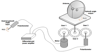
The position control of antenna through the usage of gears and feedback potentiometers is performed. Antenna azimuth position control system is currently available together with some control methods, some of the continuous PID and the discrete PID controller designed in Matlab/Simulink environment is used for controlling the position of an antenna in a spherical coordinate system called azimuth [9].
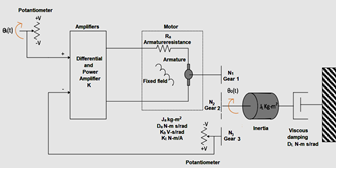
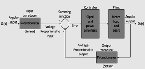
System concept of an antenna azimuth position control system is shown in Fig. 1. Analysis of model dynamics is shown in Fig. 2, Fig. 3, Fig. 4.
From Fig. 4, we have the system transmission function of the antenna system is:
| (1) |
With identified parameters shown in Table 1.
Parameters | Value |
Kpot | 0.318 |
Ki, Kp, Kd | The factors controller |
K1 | 100 |
a | 100 |
Km | 2.083 |
am | 1.71 |
Kg | 0.1 |
Here the authors selects the PID controller continuously with three factors Kp, Ki, Kd [10]-[13]. The system is simulated in Matlab as follows. If we ignore the two factors Ki, Kd, and only take Kp as 100 than we have:
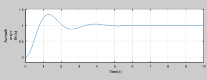
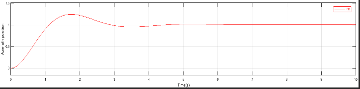
As observed in Fig. 5, the system exhibits an overshoot of approximately 25% and a settling time of around 5 sec. Furthermore, very few oscillations are noticeable in the system's response [14]. By utilizing a PID controller, the goal is to achieve improved system feedback, and the outcomes of these controllers will be compared. Thus, the above Kp =100 value can take Kc = 168.5, we find the value of Tc in Fig. 5 by measuring the period from one peak to another by 2s. The values of Kp, Ti and Td are then established according to Table 2 according to the Ziegler–Nichols second method mentioned in [14], by substituting each Kc and Tc. We get Kp=60, Ti=1, Td=0.125. It is worth saying that the obtained values of Kp, Ti and Td cannot be considered optimal, and in order to achieve the best performance of the system, more adjustments are required. The type of PID controller can be selected depending on the application of the system and the goals of the designer [15]-[17]. Than we have the result shown in Fig. 6.
Control Type | Kp | Ti | Td |
P | 0.5 Kc | - | - |
PI | 0.45 Kc | 0.83 Tc | - |
PID | 0.6 Kc | 0.5 Tc | 0.125 Tc |
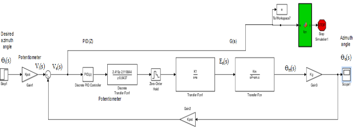
In discrete control, we choose sample time is 0.1s due to opinion that the motion of antenna should be fast to adapt the environment. Parameters of the discrete PID controllers for the antenna system shown in Table 3. Fi Here, when switching to discrete, we add noise signal:
Parameters | Value |
Kpot | 0.318 |
Ki, Kp, Kd | The factors controller |
K1 | 100 |
a | 100 |
Km | 0.8 |
am | 1.32 |
Kg | 0.2 |
Sample time | 0.1 |
| (2) |
With k is matrix [Ki Kp Kd], we have simular from Matlab shown in Fig 7. If we ignore the two factors Ki, Kd, and only take Kp as 100 than we have:
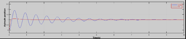
As observed in Fig. 8, the system exhibits an overshoot of approximately 35% and a significantly longer settling time, approximately 10 seconds. Furthermore, the system displays significant oscillations in its response, which can easily lead to instability if not optimized. By utilizing controller parameter optimization solutions, the goal is to achieve improved system feedback, and the results of these controllers will be compared with the optimized parameter sets. Similarly, using the 2 Ziegler-Nichols method, mentioned in [18] with a sampling time of 10 s we get Kp=60, Ki=60, Kd=15. Applying the simulation we get the result that can be seen in Fig. 9.
GAs are the optimal searching algorithm that model the evolution of biological life in nature including:
When applying the GA algorithm, we first encode the solution of the problem into a chromosome sequence (CS). Depending on the encoding method, the CS can be in the form of binary, decimal, natural number, or real number sequences. Each CS represents an individual in the population.
We define a fitness function to evaluate individuals, typically the function we want to optimize or an equivalent transformation of it. GA flowchart used in control optimization shown in Fig. 10.
The first generation is randomly initialized as a population. Through natural selection, the fittest individuals in the environment (those with high fitness) survive. This process is performed by genetic operators after ranking their fitness. Individuals with higher fitness have a greater chance of survival and are paired with others to produce the next generation.
In conjunction with selection, the crossover process has brought forth favorable traits to pass on to the next generation. Occasionally, due to errors in the natural genetic process, mutations occur. This phenomenon gives rise to individuals with lower fitness, but it can also create individuals with very high fitness.
Individuals with lower fitness are eliminated during the selection process. Through evolution, characteristics are iteratively passed from one generation to another. As a result, the subsequent generation tends to adapt better to the environment than the previous generation. This implies that the problem has an increasingly optimal solution.
Within the scope of this article, the authors employ GA with the support of MATLAB 2017 [19]-[20]. This article does not intend to introduce the GA itself. Instead, it is utilized as a tool to address optimization problems, aiming to optimize the control system's parameters (Kp, Ki, Kd). The parameters chosen for implementing GA are as follows:
Population size : n = 100
Linear selection : ƞ = 0.2
Cross coefficient : α = 0.8
Mutation parameter : β = 0.5
Significant coefficient : 0.2
The number of trainings : Max_gen = 50
Crossover probability : Pc = 0.5
Mutation probability : Pm = 0.5
Select indicator coefficient:
(3) |
e is the set error of the transfer function. The results we find through GA are set of parameters: Continuous PID controller Kp=495.7000; Ki =11.1600; Kd=101.2300; Discrete PID controller Kp = 39.3930; Ki =0.7720; Kd = 43.0060.
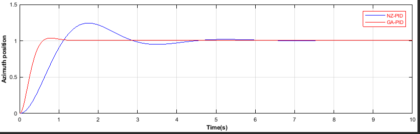
After estimating the PID parameters using the Kp selection method and optimizing PID through the GA algorithm for both continuous and discrete PID forms in two models (Fig. 11 and Fig. 12), we obtain the following comparison table. Continuous PID controller:
Discrete PID controller:
According to Table 4 and Table 5, we see that the output response on the simulation shows that the system is stable around the stability point. Optimizing continuous PID and discrete PID controllers using the GA method gives better response, significantly reduces overshoot, and increases system stability compared to the Nicola-zeller method. Continuous PID optimization method and discrete PID controller using GA are shown to perform well in simulation.
Criteria | PID-Cons | GA-PID-Cons |
Overshoot (%) | 35 | 5 |
Rise time (s) | 5 | 0.5 |
Settling time (s) | 5.6 | 0.6 |
Criteria | PID-Dis | GA-PID-Dis |
Overshoot (%) | 25 | 35 |
Rise time (s) | 2 | 0.2 |
Settling time (s) | 3 | 0.3 |
In this paper, we focus on antenna model and apply continuous and discrete PID to control position on it. GA-popular searching algorithm- is used to optimize these kinds of controllers. Simulation results show that PID classical which is found by empirical test is worse than GA-PID. Thence, this research confirms the efficiency of using GA in optimizing control parameters for both continuous and discrete PID algorithm. This is a more general than most others studies which do not recognize continuous or discrete structure in PID control.
Binh-Hau Nguyen, Application of Genetic Algorithm for Optimizing Continuous and Discrete PID to Control Antenna Azimuth Position