Journal of Fuzzy Systems and Control, Vol. 2, No 1, 2024 |
Modeling and Optimal Control for Two-Wheeled Self-Balancing Robot
Quoc-Thinh Do 1, Van-Thanh Tran 2,*, Minh-Thai Ngo 3, Minh-Quan Tran 4, Quan-Linh Thiem 5, Hoang-Son Nguyen 6,
Ba-Khoi Pham 7, Nguyen-Phuoc-An Phan 8, Duy-Hieu Nguyen 9, Duc-Hoc Nguyen 10, Van-Hoc Nguyen 11,
Ho-Minh-Quang Tran 12, Thi-Hong-Lam Le 13
1,2,3,4,5,6,7,8,9,10,11,12,13 Ho Chi Minh City University of Technology and Education (HCMUTE), Vietnam
Email: 1 19151293@student.hcmute.edu.vn, 2 19151287@student.hcmute.edu.vn, 3 19161161@student.hcmute.edu.vn,
4 20142070@student.hcmute.edu.vn, 5 19145070@student.hcmute.edu.vn, 6 19142090@student.hcmute.edu.vn,
7 20161215@student.hcmute.edu.vn, 8 20142273@student.hcmute.edu.vn, 9 20145502@student.hcmute.edu.vn,
10 20142336@student.hcmute.edu.vn, 11 20142335@student.hcmute.edu.vn, 12 20145590@student.hcmute.edu.vn,
*Corresponding Author
Abstract—The two-wheeled self-balancing robot based on an inverted pendulum model is a nonlinear object with uncertain parameters that are difficult to control with 6 state variables. This is a multiple input-multiple output (MIMO) under-actuated system that is very complex and causes many challenges for the operator. This paper analyzed the mathematical equation of a two-wheeled self-balancing robot vehicle system. Then, the Linear Quadratic Regulator (LQR) control is applied to the system through simulation on Matlab/Simulink and experiment. The results show that the LQR algorithm has been successfully applied in many moving cases.
Keywords—Two-Wheeled Self-Balancing Robot; MIMO; Optimal Control; LQR Control; Under-Actuated System
One of the research directions of the automatic control subject is the control algorithms. The two-wheeled self-balancing robot is one of the control topics related to DC motors [1]-[3]. This is a relatively classic control object in research laboratories. However, most studies are only based on simple mathematical equations with the system input being left or right wheel torque and only completed on simulation [4]-[6], while in the real model, the input is the voltage supplied to the left or right wheel motor (more complex system mathematical equation). Besides, studies applying PID, Fuzzy algorithms that are not based on mathematical models will produce system stability results that are not guaranteed by mathematics [7]-[9]. Therefore, establishing a detailed mathematical model with voltage control input is necessary. Once the detailed mathematical equation has been established, an optimal control algorithm (LQR) is the best solution to control the system because the stability of the system is guaranteed by solving the Riccati equation [10]-[12]. However, in these studies, the only simulation result is shown, and control inputs are moments of the motor. In [13], and [14], experimental models are presented. However, only stabilizing LQR control at equilibrium point is proved in that research. The survey of turn right-left is not completed. In [15], a LQG (developed from LQR method) is also proved in balancing at equilibrium point of this model. But the survey of other cases of turning left-right is not mentioned.
In this paper, the authors conducted verification through simulations on Matlab/Simulink and experiments. The obtained results show that the LQR algorithm has been successfully applied to a two-wheeled self-balancing robot in cases of balancing, turning right, and turning left.
The next sections of the article are presented as follows: Section II will discuss how to model a self-balancing two-wheeled vehicle system. Next, section III will present the optimal control algorithm applied to this vehicle system. Then, sections IV and V present the simulation and experimental control results, respectively. Finally, section VI provides conclusions.
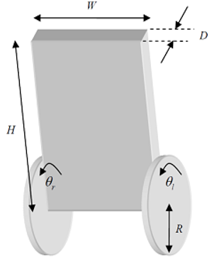
The diagram and reference system of the self-balancing two-wheeled vehicle system are shown in Fig. 1 and Fig. 2, respectively. In particular, components of system are listed in Table 1.
Notation | Unit | Meaning |
M | Kg | Mass of the wheel |
m | Kg | Mass of the robot |
R | m | Radius of the wheel |
W | m | Width of the robot |
D | m | Horizontal of the robot |
H | m | Height of the robot |
L | m | Distance from robot center of gravity to wheel axis |
fw | Coefficient of friction between the wheel and the moving surface | |
fm | Friction coefficient between robot and DC motor | |
Jm | 𝑘𝑔. 𝑚2 | Moment of inertia of DC motor |
Rm | Ohm | DC motor resistance |
Kb | V sec/rad | EMF coefficient of DC motor |
Kt | Nm/A | Torque of DC motor |
N | Deceleration ratio | |
G | 𝑚/𝑠2 | Gravitational acceleration |
𝜃 | Rad | Average angle of left and right wheels |
𝜃l,r | Rad | Angle of left and right wheels |
𝜓 | Rad | Tilt angle of the robot body |
𝜙 | Rad | Rotation angle of the robot |
𝑥l, 𝑦l, 𝑧l | M | Left wheel coordinates |
𝑥r, 𝑦r, 𝑧r | M | Right wheel coordinates |
𝑥m, 𝑦m, 𝑧m | M | Average coordinates |
𝐹𝜃,𝐹ψ,𝐹𝜙 | Nm | Moments act in different directions |
𝐹l,r | Nm | Starting moment of left and right wheel motor |
We use the Euler-Lagrange method to build the dynamic model. Supposing that at time t = 0, the robot moves in the positive x-axis direction, we have the equations below. The average translation angle of the two wheels and the rotation angle of the robot are determined as follows:
| (1) |
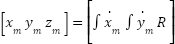
The average coordinates of the robot in the frame reference are:
| (2) |
and
| (3) |
Coordinates of the left wheel in the frame reference are:
| (4) |
Coordinates of the right wheel in the frame reference are:
| (5) |
Coordinates of the center of symmetry between the two motors in the frame reference are:
| (6) |
Kinetic energy of translational motion is
| (7) |
Kinetic energy of rotation is
| (8) |
Where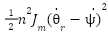 ;
; 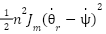 is the rotational kinetic energy of the left and right motor armatures. Potential energy is:
| (9) |
Lagrangian operator is:
| (10) |
| (11) |
| (12) |
| (13) |
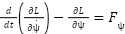
Derivating L with respect to the variables, we obtain
| (14) |
| (15) |
| (16) |
Dynamic torques produced by DC motors are:
| (17) |
Where 
Using the Pulse Width Modulation (PWM) method to control the motor, we need to convert from torque to motor voltage through this formula:
| (18) |
Assuming the armature inductance is relatively small (close to 0), it can be ignored and deduced:
| (19) |
From there, torques are generated as:
| (20) |
| (21) |
| (22) |
Where  và
và 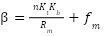 Thence, we obtain the dynamic equations describing the robot's motion as follows:
| (23) |
| (24) |
| (25) |
From (23), (24), (25), we have a system of equations describing a balanced two-wheeled vehicle system of the following form as:
| (26) |
Where
| (27) |
If we choose the working point as:
| (28) |
Then, we can linearize the system in form:
| (29) |
Where  ;
; 
At this point, we have the following weight matrices:
| (30) |
With parameters Q1 to Q6, R1 and R2, we adjust the LQR controller. Parameters Q1, Q2, Q3, Q4, Q5, and Q6 are the optimal weights for variables θ, θ, ψ, ψ, φ ,φ . A control signal for advance angle and a control signal for the rotation angle. If we want a state variable to have priority in control, we make that corresponding weight parameter relatively larger than the other weight parameters. As for the R matrix, the selection of R1 and R2 must be equal because the two wheels are proportional to each other. On the other hand, if the R matrix parameter is chosen too large, the two-wheel control signal will be strong, and responsive but sometimes unstable. If R matrix parameter is small, the model runs more smoothly. However, in some cases, it does not respond quickly and strongly enough to control the system. After selecting the corresponding control parameters, we proceed to build the feedback parameter K with the control signal.
| (31) |
Parameter K is calculated based on the Riccati equation. However, Matlab supports the lqr() function to calculate the parameter K when the matrices A, B, Q, and R as
| (32) |
The model parameters are selected as follows: m=0.037; M=0.037; R=0.035; W=0.15; D=0.075; H = 0.15; L=0.075; fw=0.18; fm=0.002; Jm=0.01; Rm=50; Kb = 0.043; Kt = 0.166; n = 21.3; g = 9.81. The weight matrices are chosen as follows:
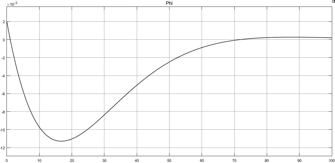
The LQR structure in Fig. 3 can be described in Matlab/Simulink program of simulation as in Fig. 4. In block that simulats the two-wheeled slef-balancing cart, smaller blocks in Fig. 5 describe this system from equations (23)-(25). The simulation results are shown in Fig. 6, Fig. 7, and Fig. 8.
| (33) |
We can calculate the K matrix as follows:
| (34) |
From results from Fig. 6, Fig. 7, and Fig. 8, the vehicle's state always follows the set signal, and the LQR controller responds quite well. Vibration is less than 0.1 degree and settling time is 60s. This proves that we can control the car in many different situations such as: driving the car forward and backward, turning left, and turning right.
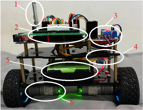
The experimental model is shown in Fig. 9. The model includes:
Optimizing the weight matrices Q and R can be done by applying genetic algorithm (GA). In this project, the team adjusted the K matrix parameters many times and produced the following results. After adjustment, the K matrix is:
| (35) |
The tilt angle fluctuates between -3 and 3 degrees, and the rotation angle and wheel angle fluctuate around the balance position. The two motor speeds are equivalent. The vehicle is stable and balanced. In Fig. 10, the body of robot is kept balanced at upward position with vibration is around -5 degrees and 5 degrees. The robot has self-balanced for more than 60s.
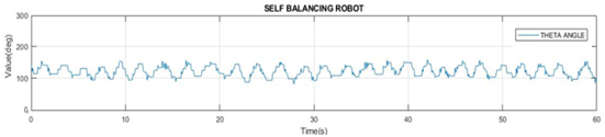
In Fig. 11, the wheel angle oscillates around the equilibrium position with vibrations of about 100 degrees and 150 degrees. Robot is stabilized at position which is in front of the equilibrium position on plane. In Fig. 12, the rotation angle oscillates around the equilibrium position with vibrations of about -2 degrees and 2 degrees. The cart is kept no rotating. Thence, in this experiment, robot is controlled well by PID method to be balanced at equilibrium point.
Experiment 1: Forward control. During the period from 53s to 66s, we change the set value to let the car move forward. Fig. 14 shows that the wheel angle points upward but still maintains the vehicle's tilt and rotation angle around the equilibrium position as shown in Fig. 13 and Fig. 15.
In Fig. 13, the body of robot is kept balanced at upward position with vibration is around -5 degrees and 5 degrees. In Fig. 14, in the period from 53s to 66s, the set value is changed, the wheel angle is directed upward.
In Fig. 15, the rotation angle oscillates around the equilibrium position with vibrations of about -2 degrees and 2 degrees. Experiment 2: Backward control. During the period from 44s to 65s, we change the set value to drive the vehicle in reverse. Fig. 17 shows that the wheel angle points downward but still maintains the vehicle's tilt and rotation angle around the equilibrium position as shown in Fig. 16 and Fig. 18.
In Fig. 16, the body of robot is kept balanced at upward position with vibration is around -6 degrees and 6 degrees.
In Fig. 17, in the period from 44s to 65s, the set value is changed, the wheel angle is directed downward.
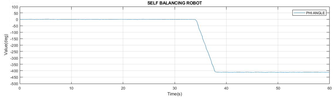
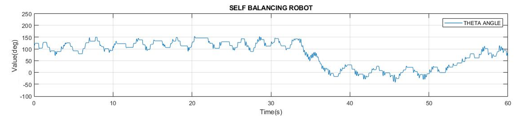
In Fig. 18, the rotation angle oscillates around the equilibrium position with vibrations of about -2 degrees and 2 degrees. Experiment 3: Control turning left. At the time of impact on the set value (from 34s to 38s), Fig. 21 shows that the rotation angle is downward but still maintained the tilt angle and wheel angle around the equilibrium position as Fig. 19 and Fig. 20. In Fig. 19, the body of robot is kept balanced at upward position with vibration is around -5 degrees and 6 degrees.
In Fig. 20, during the period from 34s to 38s, the set value is changed, the wheel angle is directed upward and the body of robot is kept balanced with vibration is around 5 degrees and 75 degrees. In Fig. 21, in the period from 34s to 38s, the set value is changed, the wheel angle is directed downward. Robot is controlled well to turn left by changing rotational angle.
Experiment 4: Control turning right At the time of impact on the set value (from 33s to 37s), Fig. 24 shows that the rotation angle is upward but still maintained the tilt angle and wheel angle around the equilibrium position as shown in Fig. 22 and Fig. 23. In Fig. 22, the body of robot is kept balanced at upward position with vibration is around -5 degrees and 5 degrees.
In Fig. 23, during the period from 33s to 37s, the set value is changed, the wheel angle is directed downward and the body of robot is kept balanced with vibration is around -25 degrees and 25 degrees. In Fig. 24, in the period from 34s to 38s, the set value is changed, the wheel angle is directed upward. Robot is controlled well to turn right by changing rotational angle.
In this project, an LQR controller is successfully designed for a self-balancing two-wheeled vehicle system - a complex and familiar MIMO nonlinear system in laboratories. The authors also successfully applied the simulation results to a realistic two-wheeled balance vehicle model using Arduino Mega 2560 microcontroller. LQR controller was tested through many cases: balancing at equilibrium point, positioning forward and backward, turning right, and turning left. It can be seen that in most cases, the LQR controller is successful in stabilizing the system and gives quite good control results. Accordingly, self-balancing two-wheeled vehicle model is a suitable model to verify and compare control algorithms, especially nonlinear algorithms.
Quoc-Thinh Do, Modeling and Optimal Control for Two-Wheeled Self-Balancing Robot