Trajectory Tracking using LQR Control for Pendubot: Simulation and Experiment

Trong-Bang Tran 1,* , Hoang-Thien Nguyen 2, Tay Nguyen 3, Duc-Dat Dang 4, Duong-Minh-Quang Pham 5,

Nhat-Duy Le 6, Hoang-Khuong Huynh 7, Thanh-Quoc-Du Phan 8, Bao-Huy Nguyen 9,

Ngo-Huu-Tung Nguyen 10, Le-Quoc-Toan Pham 11, Trung-Hieu Nguyen 12, Quang-Vinh Dang 13

1 Viet Solution Technology Technical Company Limited, Vietnam

2,3,4,5,6,7,8,9,10,11,12,13 Ho Chi Minh City University of Technology and Education (HCMUTE), Vietnam

Email: 1 bangtautomation@gmail.com, 2 20142415@student.hcmute.edu.vn, 3 20161132@student.hcmute.edu.vn,

4 20161176@student.hcmute.edu.vn, 5 20142392@student.hcmute.edu.vn, 6 20142295@student.hcmute.edu.vn,

7 20142351@student.hcmute.edu.vn, 8 20161057@student.hcmute.edu.vn, 9 20142338@student.hcmute.edu.vn,

10 20142150@student.hcmute.edu.vn, 11 20142430@student.hcmute.edu.vn, 12 20142329@student.hcmute.edu.vn,

13 20161281@student.hcmute.edu.vn 

*Corresponding Author

Abstract—Pendubot, a unique single-input-multiple-output (SIMO) system, is commonly employed in laboratories to validate control algorithms. In this article, we develop an LQR controller to simulate and assess its effectiveness on this model. Specifically targeting the TOP position for control, we not only verify the controller's quality but also ensure the motion system accurately tracks a predefined trajectory, encompassing sine and square pulses. Control parameters are meticulously chosen through a genetic algorithm (GA). Although LQR is not highly rated for trajectory tracking due to its relatively small operational range, our successful simulations and control of this system are attributed to the assistance of GA.

Keywords—Pendubot; LQR Control; SIMO System; Stabilize Control; Genetic Algorithm

1. Introduction

Pendubot, formally known as Pendulum Robot, serves as a standard and classic model system with a significant role in algorithm research at automatic control laboratories. Studying algorithms on standard models like the Pendubot provides students with valuable learning and training opportunities. Armed with this knowledge, students can later apply these algorithms to real-world scenarios during their work. Examples include implementing balancing systems for offshore drilling rigs, ensuring stability during spacecraft launches, and controlling their trajectories accurately.

In [1], the author introduced the mechanical structure of pendulous. This marks the first research work by a Vietnamese author on this mechanical structure. LQR [2] and PID [3] algorithms were chosen to control the balance of this system. The controller exhibits very good quality, but this outcome is based on simulation, and there is no model available to verify the quality. Although experiments on the model can be easily found on platforms like YouTube, they often stop at static positions, such as TOP (both link 1 and link 2 up) or MID (link 1 down and link 2 up). In the document [4], the experiment of swinging up and balancing control at a static position is presented. Another published nonlinear controllers, such as Sliding Mode Controller [5], Fuzzy controller [6] based on 81 rules in [7], back-stepping [8] or controller combined of 2 controllers: adaptive Fuzzy  PID [9], adaptive Fuzzy Sliding Mode [10],  adaptive Fuzzy Hierarchical Sliding Mode [11],  LQR base on Fuzzy logic control [12] demonstrate impressive results with a large working area in simulation. However, the related published documents are not fully verified, and numerous issues arise when simulating to find parameters for the controller. Basically, every controller needs suitable parameters found based on experiments from experts or the workspace. Moreover, GA [13] and PSO [14] were recommended to support experts do it.

In this article, an LQR controller will be chosen for experimental verification with more challenging working positions to ensure more rigorous validation. Simultaneously, we have enhanced the accuracy of the simulation verifications to obtain a set of control parameters suitable for the existing hardware, aiming to make the simulation as close to the experiment as possible.

2.  Mathematical Model

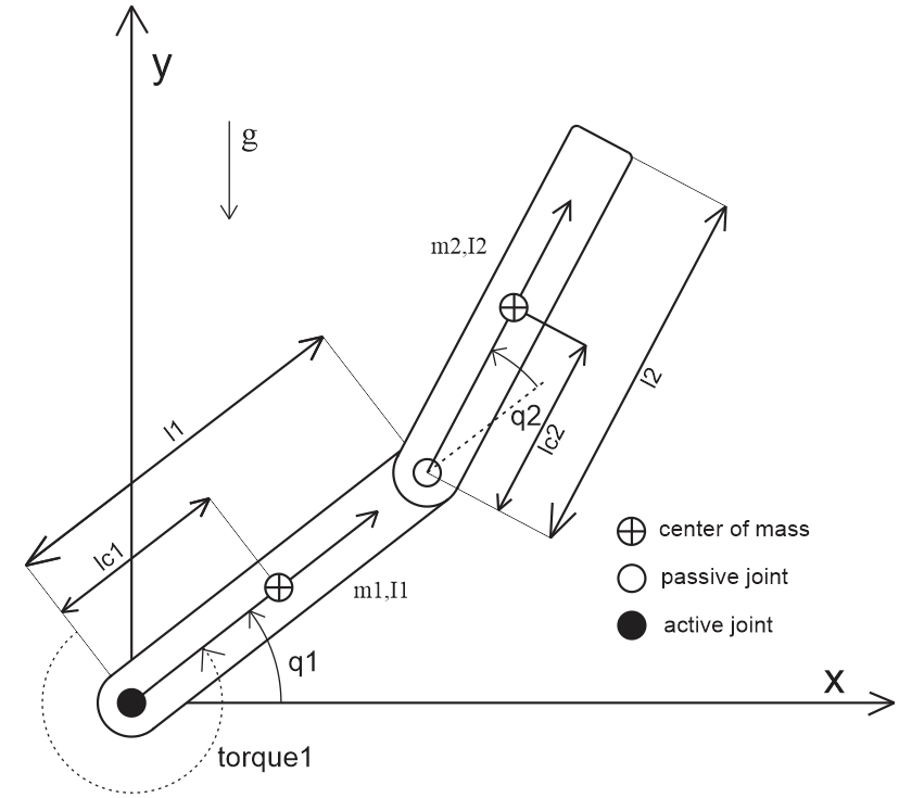
A pendubot consists of two bars linked together in a plane by a free joint, Fig. 1. Link 1 is connected to a motor that balances link 2 at two experimentally controllable positions: TOP and MID, as described in [12]. In the TOP position, both links point upwards, while in the MID position, link 1 down, and link 2 up. Table 1 list the system parameters used.

1. System minimum of the proposed system

From [1], the mathematics of the system is rewritten as:

Where: ; ; ; ; .

1. System parameters

Linear equations have the form: Where:

3. Controller Method

According to our experience, the ideal sampling time is 5ms. Matrices A and B are continuous. Thence, we need to convert it to the discrete system by MATLAB command:

The equilibrium point is chosen as:

This equilibrium point is the TOP position of Pendubot. At that position, the moment on link 1 is zero to maintain the system stability.  If the system is the round working point in (5), the LQR signal to the control system is:

Basically, weighing matrixes Q and R can be selected as eye matrix. However, the simulation we designed is not ideal with resolution-limited hardware. There for, the genetic algorithm (GA) is used to find and optimize these matrixes.

Matrix K is calculated by Matlab command:

4. Genetic Algorithm

Based on thesis from document [7] and objective function in document [10], we choose configuration parameters for GA.

• Maximum number of generations: 200;
• Number of individuals: 50;
• Hybridization coefficient: 0.8;
• Mutation coefficient: 0.2;
• Encoding type: binary encoding;

With the search results demonstrating excellent control quality in the document [10], the objective function is selected as follows:

Where the objective function variables are explained in Table 2.  These values will be collected continuously throughout the simulation.

2. Variables for the objective function

5. Simulation

To simulate and verify the quality of the controller. We need to set the initial state of the system. The parameters are selected as Table 3.

3. Initial state values

These initial values are chosen to be relatively large with the aim of expanding the workspace. Similarly, the parameters identified through GA can ensure quality control. Fig. 2 shows the MATLAB Simulink of the system used.

2. Simulation simulink program

Detailed description: The largest block, labeled “pendubot”, describes the state of pendubot. We have slightly adjusted it to represent the data status that the microprocessor reads from the experimental model. The “LQR” block contains Equation (6). The 'limit' block constrains the torque to the correct torque limit of the motor we have selected. The “sample trajectory” block holds the working trajectory that we have designed. The “error” block is designed to trigger an interruption in case the system becomes unstable. The data “e”, “e1” and “e2” are stored for use in the GA loop.

Detailed description: In Fig. 3, we do not directly utilize the system's state variables due to the lag between the real model's velocity and the reading time. Therefore, we differentiate the angle reading value to obtain the state value that closely resembles the experimental model. After 1000 generations of GA searching, we found a suitable K Matrix set as follows:

3.  “Pendubot” block

Matrix (4) is a constant. By substituting (9) into (8), we obtain the following control matrix:

With the aim to optimize both results and energy consumption for increased feasibility in experiments, achieving about 90% of the sample trajectory in simulation results is a very positive outcome. The angular state  shown in Fig 4.

4. The angular state  compared to the sample

6. Experiment

Fig. 5 shows the real pendubot used in this study. In the experiment, we increased the amplitude of the sample trajectory to clearly differentiate it from the stable TOP position. Equipment is selected and used for experiments:

With a simulated torque limit of 0.5N, the motor in Fig. 6 meets the requirements, provided the power supply reaches the minimum voltage as shown in Fig. 7. To adjust and modulate the pulse to match the consumption level, the H-bridge circuit in Fig. 8 ensures signal quality and transmission efficiency. The selected microprocessor in Fig. 9 operates at a maximum clock speed of 72MHz, ensuring prompt signal reading from a high-resolution encoder with up to 600 pulses in Fig. 10 and processing data promptly within a 5ms sampling time. To load the program into the microprocessor, you need to use a downloader circuit as shown in Fig. 11. During the experiment, data will be returned to the computer via the UART communication standard, so an additional circuit is needed to translate from UART to USB standard as shown Fig. 12 for the computer to read.

5. Experimental pendubot model

6. DC NISCA Servo Motor NF5475E

With this controller, we need to convert torque into a voltage signal. From the document [15], we have a formula (11). The engine parameters we identify are listed in Table 4.

4.         Engine parameters

Unlike simulating, variables with high resolution up to 32 bits, where the smallest changes are eliminated immediately. In experiments, the resolution of the angular value and angular velocity readings depends on the number of pulses from the encoder. This ensures that resulting signal spikes do not lead to chattering. The angular state  compared to the sine wave shown in Fig. 13. The angular state  compared to the pulse shown in Fig. 14.

7. The angular state  compared to the sine wave. This experiment is equivalent to the simulation of Fig. 4 from 0 seconds to 140 seconds

8. The angular state  compared to the pulse. This experiment is equivalent to the simulation of Fig. 4 from 150 second to 300 second

The ability to track the trajectory is quite good but requires substantial hardware, including a high-resolution encoder for prompt system status feedback. Additionally, the microprocessor must process information swiftly to avoid missing the encoder's signals.

Through two types of orbits, it can be observed that, despite being a linear controller, LQR effectively governs a nonlinear system along a nonlinear trajectory. However, it is still capable of stabilizing the system in static positions and following dynamic trajectories. The experimental values unmistakably showcase the unexpected capabilities of the LQR optimal controller. More details are shown in the links of YouTube: Sine wave: https://youtu.be/dVe7zvcfW-0. Pulse wave: https://youtu.be/WrvH5jD5KTg

7. Conclusion

In general, even though the LQR controller is designed for linear systems, its control parameters are derived from mathematical equations. The controller demonstrates an ability to handle situations beyond the nominal working position, such as in the TOP position. This suggests that with a comprehensive understanding of the system's mathematical equations and parameters, LQR stands out as a controller that ensures quality and is easily accessible.

Acknowledgement

We want to give thanks to the Ph.D. Van-Dong-Hai Nguyen (Faculty of Electrical and Electronics Engineering – HCMUTE) due to his supervision in this contribution.

References

1. M. Zhang and T. Tarn, “Hybrid control of the Pendubot,” IEEE/ASME Transactions on Mechatronics, vol. 7, no. 1, pp. 79-86, 2002, https://doi.org/10.1109/3516.990890.
2. V. -D. Nguyen et al., “Optimal Control of Pendubot System using SIMATIC S7-1200,” International Journal of Robotica & Management, vol. 28, no. 1, pp. 43-52, 2023, https://doi.org/10.24193/rm.2023.1.6.  
3. R. P. Borase, D. K. Maghade, S. Y. Sondkar, S. N. Pawar, “A review of PID control, tuning methods and applications,” International Journal of Dynamics and Control, vol. 9, pp. 818-827, 2021, https://doi.org/10.1007/s40435-020-00665-4.
4. X. Yu, Y. Feng and Z. Man, “Terminal Sliding Mode Control – An Overview,” IEEE Open Journal of the Industrial Electronics Society, vol. 2, pp. 36-52, 2021, https://doi.org/10.1109/OJIES.2020.3040412.
5. I. Chawla, A. Singla, “Real-time stabilization control of a rotary inverted pendulum using LQR-based sliding mode controller,” Arabian Journal for Science and Engineering, vol. 46, pp. 2589-2596, 2021, https://doi.org/10.1007/s13369-020-05161-7.

6. C. Wei, T. Chai, X. Xin, X. Chen, L. Wang and Y. -H. Chen, “A Signal Compensation-Based Robust Swing-Up and Balance Control Method for the Pendubot,” IEEE Transactions on Industrial Electronics, vol. 69, no. 3, pp. 3007-3016, 2022, https://doi.org/10.1109/TIE.2021.3065621.
7. M. Mao, L. Cui, Q. Zhang, K. Guo, L. Zhou, H. Huang, “Classification and summarization of solar photovoltaic MPPT techniques: A review based on traditional and intelligent control strategies,” Energy Reports, vol. 6, pp. 1312-1327, 2020, https://doi.org/10.1016/j.egyr.2020.05.013.
8. L. Guoping, X. Genfu and Y. Xiaohui, “The LQR Real-time Control for the Inverted Pendulum Based on PSO,” 2010 International Conference on Electrical and Control Engineering, pp. 2363-2366, 2010, https://doi.org/10.1109/iCECE.2010.583.
9. L. T. Le, H. Nguyen, J. Dou, J. Zhou, “A comparative study of PSO-ANN, GA-ANN, ICA-ANN, and ABC-ANN in estimating the heating load of buildings’ energy efficiency for smart city planning,” Applied Sciences, vol. 9, no. 13, p. 2630, 2019, https://doi.org/10.3390/app9132630.
10. J. Wu, Y. Wang, W. Ye, C. Y. Su, “Control strategy based on Fourier transformation and intelligent optimization for planar Pendubot,” Information Sciences, vol. 491, pp. 279-288, 2019, https://doi.org/10.1016/j.ins.2019.03.051.

11. R. A. Maafi, S. E. Haghighi, M. J. Mahmoodabadi, “Pareto optimal design of a fuzzy adaptive hierarchical sliding-mode controller for an XZ inverted pendulum system,” IETE Journal of Research, vol. 69, no. 5, pp. 3052-3069, 2023, https://doi.org/10.1080/03772063.2021.1910578.
12. T. N. Nguyen, P. L. Nguyen, V. D. H. Nguyen, “Pendubot Controls using LInear Quadratic Regulator Combined Fuzzy,” Dong Thap University Journal of Science, no. 38, pp. 89-93, 2019, https://doi.org/10.52714/dthu.38.6.2019.704.
13. S. Katoch, S. S. Chauhan, V. Kumar, “A review on genetic algorithm: past, present, and future,” Multimedia Tools and Applications, vol. 80, pp. 8091–8126, 2021, https://doi.org/10.1007/s11042-020-10139-6.
14. A. G. Gad, “Particle swarm optimization algorithm and its applications: a systematic review,” Archives of computational methods in engineering, vol. 29, pp. 2531-2561, 2022, https://doi.org/10.1007/s11831-021-09694-4.
15. T. D. Nguyen et al., “Feedback LInearization Control for Inverted Pendulum,” Dong Thap University Journal of Science, vol. 12, no. 2, pp. 50-58, 2023, https://doi.org/10.52714/dthu.12.2.2023.1032.