;
;  ;
; 
Journal of Fuzzy Systems and Control, Vol. 2, No 1, 2024 |
PID Control for Cart and Pole System: Simulation and Experiment
Thai-Bao Dang 1,*, Truong-Doan-Hy Ngo 2, Thanh-Danh Tran 3, Thi-Kieu-Tien Vo 4, Nguyen-Ngoc-Truc Lai 5,
Thi-My-Linh Huynh 6, Thi-My-Hang Nguyen 7, Thi-My Nguyen 8, Tuong-Vy Le 9, Khanh-Hung Pham 10,
Nguyen-Cuong Huynh 11, Anh-Tuan Nguyen 12, Thanh-Trung Nguyen 13
1 FPT Software Company, Ho Chi Minh City, Vietnam
2,3,4,5,6,7,8,9,10,11,12,13 Ho Chi Minh City University of Technology and Education (HCMUTE), Vietnam
Email: 1 baodt12@fpt.com, 2 20161056@student.hcmute.edu.vn, 3 20161169@student.hcmute.edu.vn,
4 20124164@student.hcmute.edu.vn, 5 20124200@student.hcmute.edu.vn, 6 20124275@student.hcmute.edu.vn,
7 20124179@student.hcmute.edu.vn, 8 20124220@student.hcmute.edu.vn, 9 21126107@student.hcmute.edu.vn,
10 20142343@student.hcmute.edu.vn, 11 20142290@student.hcmute.edu.vn, 12 20142077@student.hcmute.edu.vn,
13 19161184@student.hcmute.edu.vn
*Corresponding Author
Abstract—Inverted pendulum (IP) is a single input-multi output (SIMO) nonlinear system that is popular in laboratories of control engineering. In this paper, we propose a structure of the PID control method – the most popular control method in the industry - for the cart and pole (C&P) system- a kind of IP. In this case, a suitable structure can help single input-single output (SISO) linear controllers to balance well. By this combination, the PID method can be used to stabilize this model at the equilibrium point. This controller is proven to work well in simulation. Therefore, we also present an experimental model which is created from the STM32F4 Discovery board for testing this algorithm. The experiment results again confirm the suitability of the method in simulation. Therefore, a survey of PID calibration is examined. The experimental survey confirms the suitability of this PID controller with theoretical points. The results from this study can be used to examine and train algorithms for learners in control laboratories.
Keywords—Cart and Pole; Inverted Pendulum; PID Control; Linear Controller; SIMO Systems
An inverted pendulum (IP) is popularly used in control laboratories due to its simple but highly nonlinear characteristics [1][2]. C&P, also known as IP on the cart is a classical SIMO nonlinear model in many experiments about controlling theory because of its high instability [3]. The system also serves as a foundation for more complex systems like orbiting and tracking missiles, machinery axes that need to be stabilized with high precision, etc. In fact, much similar research on how to control the trajectory of IP has been carried out through the decades. It is also developed to be a standard model by Quanser company [4]. However, most of them are only conducted through simulation [5]. Many studies with a functioning model also do not implement orbital control, only placement control at a fixed point. Many researchers also use self-made models [6] controlled by algorithms such as linear controllers [7], such as PID, LQR, and pole placement. In that study, the comparison is among the linear control methods. The development of research can be fuzzy [8] or sliding mode control [9]. However, PID is still the most popular method in academies and industry [10] due to its simple structure. Moreover, the operators can neglect system information but still make the system work well through calibrations. Researchers from many universities around the world, including undergraduates, have done projects related to under-actuated systems [5], [6]. Due to the high price of C&P of Quanser [4], many experimental C&P systems are made to satisfy the requirement of control engineering research in poor countries. In [11], a hardware of DSP TMS320F28335 is used to balance well experimental C&P. However, this control board is expensive, and it is not supported freely from Texas anymore. In [12], Arduino – a popular processor- is introduced to be applied on real C&P with a PID controller. However, this processor is low-speed and has low memory. Thence, it is not suitable for intelligent and nonlinear methods. In [13] and [14], STM32F4 is proved to be a cheap, high-speed, and MATLAB-embedded processor which can be used for complicated systems. In the research, the real model is a rotary inverted pendulum (RIP) which is different from C&P. RIP is easier to control than C&P. The Operating range of the arm of RIP is larger than the operating range of the cart of C&P although the same roles.
Thence, a new control hardware platform must be considered. In this study, we build a structure of PID controllers to balance well C&P. Besides, a self-made experimental model is presented as a hardware platform that is based on STM32F4 – a new and updated control board- to develop algorithms for our laboratory.
The mathematical model of C&P is shown in Fig. 1. The pole will rotate around an axis of the encoder attached directly to the cart. We aim to keep the pole stabilized at a balanced position (upward). At the same time, the cart will also be moving along a calculated orbit so that the pole will not be able to fall below and maintain a balanced position. From [11], dynamic equations of C&P are shown in equation (1) and equation (2).
Where, L: Length of the pole (m); m: Weight of the pole (kg); M: Weight of the cart (kg); J1: Moment of Inertia (kgm2); θ: pendulum’s angle (rad); x: position of the cart (m); Rm: motor’s resistor (Ω); Lm: reactance factor (H); Eb: electromotive force (V); Jm: inertia moment of the rotor (kgm2); Kb: reactance constant (V/(rad/sec)); Kt: moment constant (Nm/A); ω: motor’s velocity (rad/s); θm: motor’s shaft rotation angle (rad); Tf: frictional moment (Nm); Cm: oil’s frictional coefficient (Nm/(rad/sec));
; ;
| (1) |
| (2) |
Re-writing the dynamic equations into matrices, we obtain.
| (3) |
where: 
By defining variables, we obtain a matrix of varies as follows:
| (4) |
Equation (3) becomes:
| (5) |
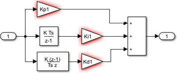
C&P is a SIMO system. However, the PID controller is a SISO structure. Therefore, we propose a structure of double- ID controller structure which is shown in Fig. 3. Inside each PID block, the description is shown in Fig. 2.
By obtaining system parameters from the real model, we have. These parameters are the same in both simulation and experiment. The simulation program is described in Fig. 3. The simulation process is divided into 3 cases: balancing at the equilibrium point, following sine trajectory, and pulse trajectory. Control parameters are found by GA as the method in [15]. Simulation responses of the system are listed from Fig. 4 to Fig. 9.
| (6) |
By using GA combined with PID, we obtained the following PID parameters:
| (7) |
Fig. 4 and Fig. 5 show that the PID controller can stabilize the system at the balanced working point. The pole’s angle is driven to zero, while the cart’s position is heading to the set point, which in this case is 0.08. The cart nearly stands still while the pole is in a vertically upward position. The settling time is 4 sec.
By using GA combined with PID, we obtained the following PID parameters:
| (8) |
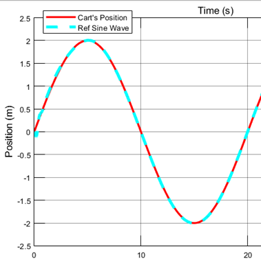
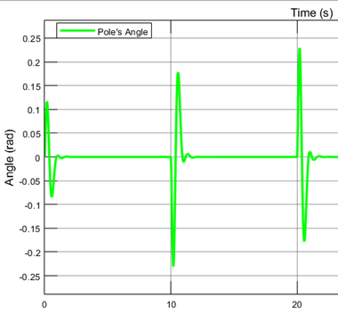
We provide a sine wave input for the system that acts as an orbital reference sample. The cart will move according to the value of the sine wave while trying to keep the pendulum in a vertically upward position. Fig. 6 and Fig. 7 show that the PID controller successfully controls the system. The cart follows a sine trajectory, and the pole is balanced after a short time (< 1 sec).
Similar to the previous simulation this time, a pulse (square) wave input as the orbital reference sample. This square wave has 0.2 amplitude and a 20s period. By using GA combined with PID, we obtained the following PID parameters:
| (9) |
Fig. 8 and Fig. 9 show that this system is still stable. The cart follows a square pulse trajectory while the pole remains firmly in the balanced vertically upward position. Especially we can see the cart is stable at around 4s, with low overshoot (<10%). The pole’s angle takes just under 2s to return from its current position to the balanced position. However, by reducing the square wave period by a significant amount (for example 5s period), the system is forced to adapt faster, so this could lead to some inaccurate output responses (too slow or too fast).
Our experimental model is shown in Fig. 10. The connection of hardware is shown in Fig. 11.
The structure of C&P in Fig. 10 is shown by numbers:
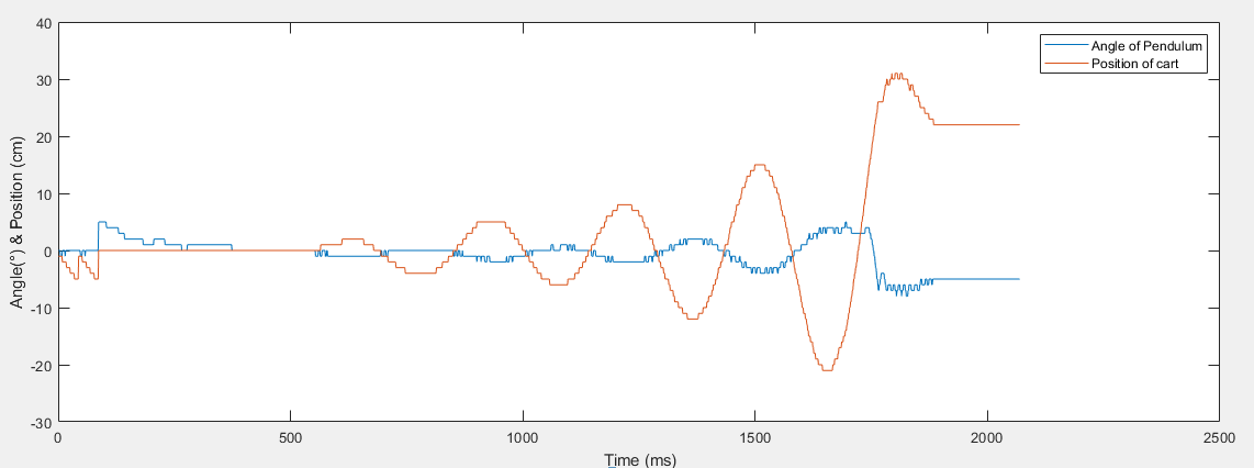
In experiments, PID parameters are re-used. The result shows the stability of the system under the control algorithm. Friction, extraneous noise, and error identification of motor parameters are additional effects that act upon the system and are ignored in simulation. However, the fact that the system still performs well proves that the PID controller has high stability. In Fig. 12, the settling time is 17 sec. The pendulum angle ranges from -20 degrees to 20 degrees. Cart position ranges from -36 cm to 36 cm. However, the oscillation of the cart is still high, and it tends to be higher and higher. Still, the system works well. Control parameters in case 2 shown in Table 1.
KP | Kd | |
Pendulum | 405 | 0.22 |
Cart | 82 | 0.11 |
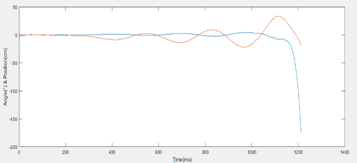
In Fig. 13, when Kp of the pendulum is reduced by 10%, the biggest change is that the actual response of the angle of the pendulum, amplitude, and frequency of operation is smaller than the student's chosen parameter. Besides, the cart still holds the position well in 11 sec. Control parameters in case 3 Table 2.
In Fig. 14, when increasing the Kp value by 10% from case 1, the angle of the pole only increases the operating amplitude around the equilibrium position, it still clings well to the equilibrium position. Besides, the cart position tends to deviate from the equilibrium point, which due to the system being less stable drops faster. Control parameters in case 3 Table 3.
In Fig. 15 when decreasing Kp value by 10%, the cart still holds the pole in the equilibrium working range. However, the oscillation of the cart increases due to the system drop in 7 sec which means too fast. First PID parameters, decreasing Kp2 by 10% from case 1 shown in Table 4.
Kp | Kd | |
Pendulum - 1 | 364.5 | 0.22 |
Cart - 2 | 82 | 0.11 |
Kp | Kd | |
Pendulum - 1 | 445.5 | 0.22 |
Cart - 2 | 82 | 0.11 |
Kp | Kd | |
Pendulum - 1 | 405 | 0.22 |
Cart - 2 | 73.8 | 0.11 |
In Fig. 16 when increasing Kp of the cart by 10%, the response of the cart increases which can keep the pole at the equivalent point 2 sec longer. The operating amplitude around the equilibrium position of the pole is the smallest and most stable. Along with that, the cart also works around the original position and does not deviate much on both sides. First PID parameters, increasing Kp2 by 10% from case 1 (case 5) shown in Table 5.
Kp | Kd | |
Pendulum - 1 | 405 | 0.22 |
Cart - 2 | 90.2 | 0.11 |
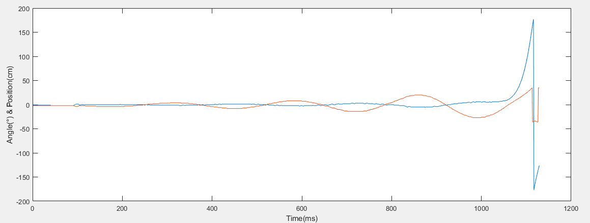
In Fig. 17 when decreasing Kd value by 10% and keeping the remaining parameters at the original, the operating amplitude around the equilibrium position of the pole and the cart is the smallest and most stable. However, at the 10th second, the cart tends to be derived from the original working point and drops the pole. First PID parameters, decreasing Kd1 by 10% from case 1 (case 6) shown in Table 6.
Kp | Kd | |
Pendulum - 1 | 405 | 0.198 |
Cart - 2 | 82 | 0.11 |
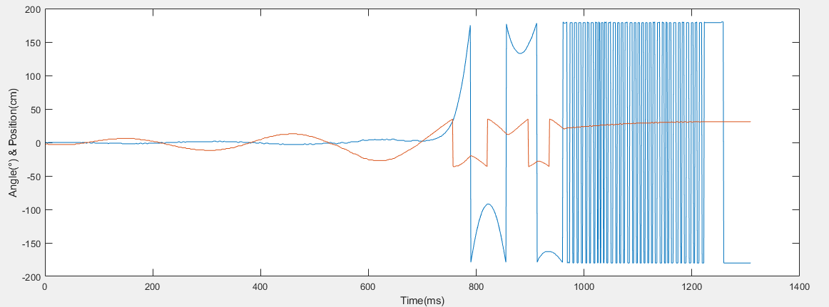
In Fig. 18 when decreasing Kd value by 10%, the operating amplitude is around the equilibrium position of the pole and the cart. The increasing of the pendulum Kp makes the cart oscillate in the wide range which due to the pendulum bar drops fast. However, the system still works well. First PID parameters, increasing Kd1 by 10% (case 7) shown in Table 7. In Fig. 19 The 10% decrement of cart Kd has significant effects on the system. It makes the cart become less stable and start to lose control after a while, while also increasing the operating amplitude around the equilibrium position. Furthermore, due to a limitation on the hardware’s part, we can only control the cart from -35 cm to 35 cm. In the figure, the cart is constantly out of bounds due to noises. This phenomenon makes this system only work in a short time which is 4 sec. First PID parameters, decreasing Kd2 by 10% (case 8) shown in Table 8.
Kp | Kd | |
Pendulum - 1 | 405 | 0.242 |
Cart - 2 | 82 | 0.11 |
Kp | Kd | |
Pendulum - 1 | 405 | 0.22 |
Cart - 2 | 82 | 0.099 |
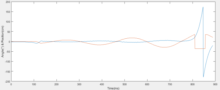
In Fig. 20 the 10% increase of cart Kd effects upon the system is stable in 7 sec. In the beginning, the cart holds the pendulum bar well. However, in the middle of the process, the oscillation is high which leads to the drop of the pendulum. First PID parameters, increasing Kd2 by 10% (case 9) shown in Table 9.
Kp | Kd | |
Pendulum - 1 | 405 | 0.22 |
Cart - 2 | 82 | 0.121 |
Based on the variation of each parameter in the first experiment, these are some conclusions:
Through this study, we examine the mathematical model of C&P with voltage as the control signal. We propose a structure of PID control to balance this model at the equilibrium point. Simulation results prove that this method is suitable to balance this system at the working point and control parameters are obtained by GA. Also, trajectory tracking control is successful with pulse and sine trajectories. We also propose an experimental C&P model using the STM32F4 discovery board. In the experiment, our control method is proven to balance C&P effectively. With this platform, we tested control rules in PID theory, and the suitability of calibration rules of PID in theory and reality is confirmed.
We want to give thanks to the Ph.D. Van-Dong-Hai Nguyen (Faculty of Electrical can Electronics Engineering – HCMUTE) due to his supervision for us in this contribution. The link to the real operation of the system is shown in the link: https://www.youtube.com/shorts/WzNs9FTrlks
Thai-Bao Dang, PID Control for Cart and Pole System: Simulation and Experiment