Journal of Fuzzy Systems and Control, Vol. 2, No 2, 2024 |
Beta-Deficient Estimators with Truncated Sampling Plan in Quality Control for the Auto Battery Industry
Salman Hussien Omran 1,* , Salam Waley Shneen 2, Mohanned M. H. AL-Khafaji 3
1,2 Energy and Renewable Energies Technology Centre, University of Technology- Iraq, Baghdad
3 Dep. of Production Engineering and Metallurgy, University of Technology- Iraq, Baghdad
Email: 1 Salman.H.Omran@uotechnology.edu.iq, 2 salam.w.shneen@uotechnology.edu.iq,
3 Mohanned.M.Hussein@uotechnology.edu.iq
*Corresponding Author
Abstract—Quality manipulation plays an essential feature in assuring product reliability and patron loyalty. Single Sampling Plans (SSPs) are usually utilized in excellent assurance to decide whether a batch of items should be popular or rejected based on sample characteristics. Truncated SSPs are a subset of those plans that offer benefits in sampling performance and price effectiveness. However, the lifestyles of outliers in accrued information will have a substantial impact on the accuracy and reliability of estimators employed in truncated SSPs. This examination explores the impact of outliers on the overall performance of truncated SSP estimators, in addition to their implications for quality control decision-making. We begin by providing a comprehensive overview of truncated SSPs and their applications in the industry. Then, at that point, delve into outlier detection methods and investigate their effectiveness in identifying potential anomalies inside tested information. Notwithstanding theoretical insights, this exploration incorporates a practical application where we exhibit the effect of outlier detection and robust estimation techniques on real-world quality control choices. By giving rules and recommendations for practitioners, this study expects to upgrade the reliability and effectiveness of truncated SSPs within the sight of outliers, eventually adding to further developed product quality and consumer satisfaction in manufacturing and other industries.
Keywords—Outliers; Truncated Single Sampling Plan; Quality Control; Batch Acceptance; Reliability; Beta Distribution
The sampling method is a suitable means for getting an estimate of the availability of one or several characteristics in the production units, by looking at an example of the total production. The task `that was embraced in the field of quality control and the concept of defective and average example size (ASN) is one of the significant attributes that should be assessed to have the option to compare with other sampling methods like single, double, sequential, and others.
In [1] presents an exploration that arrangement with presenting acceptance sampling plans is one of the statistical tools used to work on quality and control cases in which it is not possible to test all experimental units. The result of the test is the acceptance or rejection of the group based on the statistical test of a specific random sample. It is important to determine the statistical distribution of experimental units. The study included introducing a new distribution called Ishita, based on a specific period and determining the distribution parameters for the drawn sample based on taking the smallest sample size sufficient to make the decision to accept or reject the experimental units. In this study, an individual acceptance sampling plan was developed for the assumed distribution and assuming that the average age represents a predetermined parameter to measure consumer and producer risks at the same time. Based on the results, consumers and producers are advised to adopt this plan to save time and reduce the production process. Future research could be conducted on single-acceptance sampling plans assuming that products have different age distributions.
In [2], a group acceptance sampling plan was developed when following the lifeline generalized exponential logistic distribution (OGELLD) by adopting multiple parameters and as one group for the same time. The design parameters and the minimum group size were adopted, after which the test end time was determined by adopting the acceptance curve. The study included accepting the sample when the product age followed the assumed distribution, and the number of groups and the assumed number were determined to reach acceptance of the batch when taking the consumer’s risk and the producer’s risk at the same time. The results showed that the approved methodology is adopted according to the assumed data.
In [3], a sampling plan was presented for the case of mass acceptance when the lifetime of the element follows an inverse alpha distribution. The study included adopting the median as a measure to verify the quality of the sampling plan design parameters and adopting both the lower and upper limits for the group studied. Which is determined upon completion of the test? The set of operating characteristic values was presented in tabular form, relying on two test sets. In this study, the lifetime was presented by following the inverse alpha distribution and adopting the median to continue the test or stop and end up reaching a specific decision. The results showed that the optimal values tend to decrease when the corresponding values in the tables increase. Therefore, we will focus our research on estimating the defective percentage in the amputated sampling, as well as deriving the average sample size. The individual examination plan must be clarified and the amputated examination dealt with. The aim of research is to find the least sample size that satisfies the acceptance of or rejection of the lot, reducing inspection processes and truncating sample size is very useful for minimizing the cost of quality control.
Acceptance sampling is an inspection method that is widely used in vast areas of industrial application and implementations to inspect many items in a short amount of time without decreasing the quality of the items or inspection precision. It is ideal to inspect all the products manufactured in the factory line to ensure the quality of the product without nonconformities (unacceptable product quality) but it is almost impossible to inspect every product without consuming a very long time, labor costs and possibly causing human error because of fatigue and boredom that will reversely make the non-conform product miss the inspection [4].
It is a commonly used method in quality control and statistical quality assurance to determine whether a batch or lot of products meets specified quality standards. It is a type of attribute sampling plan, which means that it focuses on determining whether a discrete item or unit conforms to a set of predefined criteria, rather than measuring a continuous variable.
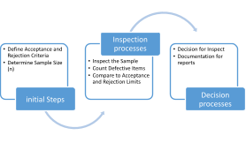
Key components of SPP, define Acceptance and Rejection Criteria: The first step in creating a single sampling plan is to establish clear criteria for acceptance and rejection. These criteria are generally characterized as far as the number of defective items permitted in an example or lot.
Determine Sample Size  : The example size is the quantity of items randomly chosen from the lot for inspection. The sample size is commonly resolved utilizing statistical tables or equations in view of variables like the desired level of confidence and the acceptable quality level.
Select a Random Example: Utilizing an arbitrary testing technique (like irregular number tables or irregular sampling software), select n things from the lot without bias. This guarantees that the sample is illustrative of the whole lot.
Inspect the Sample: Analyze every item in the sample according to the predetermined criteria. Decide if every item is acceptable or defective based on these criteria.
Count Defective Items: Ascertain the quantity of defective items in the sample.
Contrast with Acceptance and Rejection Limits: Look at the number of defective items in the sample to the predefined acceptance and rejection limits. These limits are regularly characterized utilizing statistical principles. Assuming the quantity of defects falls within the acceptance limit, the lot is accepted. Assuming it exceeds the rejection limit, the lot is rejected.
Decision: In view of the comparison, make a decision on whether to accept or reject the whole lot. The decision should be made according to the predetermined rules of the sampling plan.
Documentation: Document the results of the inspection, including the number of defects found, the sample size, and the decision made.
Single Sampling Plans are widely used in industries where discrete items are produced in large quantities, such as manufacturing, electronics, and pharmaceuticals. They provide a balance between the cost of inspection (sampling and testing) and the level of quality control required. Different sampling plans can be used based on the specific needs of a particular application, with variations in sample size, acceptance limits, and other parameters to achieve the desired level of quality assurance. The following Fig. 1 shows the Single Sampling Plans steps [5].
The truncated examination is defined as the precautionary measures in the process of taking models, to stop the examination at a point at which it becomes clear that the data collected by the researcher is appropriate for decision-making. The importance of the truncated examination appears in the case of medical experiments and in the event that the produced units are damaged during the examination, and Hald believes that in the case of a truncated examination, it is not necessary to examine all sample units to reach the decision. It is possible to obtain the same decision in the case of examination of all sample items or to interrupt the examination process in the event of obtaining  from the defective units or in the event of obtaining
  of good units. In the truncated examination, the number of examined units necessary to reach the decision is a random variable (Y) that takes values from to n or from
  and the probability function is y is the negative binomial, as will be explained later.
In the truncated examination, the examination is stopped when defective units are obtained that exceed the acceptable number or good units that are not less than are obtained. The important advantage in this type of examination is obtaining the number of plates [6].
 is the probability of testing a defective unit on the first try.
  is the total accumulated number of defective units that appear during the inspection when the payment is rejected or accepted.
  is the total accumulated number of good units for which payment is accepted.
  is the total number of examined units to reach a decision (reject or accept) on the payment, such that.
|
|
That the probability function of the variable y is a negative binomial distribution with parameter  .
.
|
with  represent reject region, with
  represent accept region
|
The probability of rejecting the lot will be [7].
| (1) |
Since
|
Then
| (2) |
Where (z) is a random variable that represents the number of defectives that appear during the examination when examining a sample of size (n) taken from a batch of size (N)
Suppose that (m) batches of size (N) were subjected to examination, according to the truncated sampling method, it was found that the number of accepted batches is (a) and the number of rejected batches is(r) [8].
And
|
During the inspection process, the number of units that were checked from each batch and the number of defective units that we obtained were recorded. According to the registration process, the sample data will be [9].
|
and
|
Represent the number of defective units in the accepted lot with, number of defective units in the rejected lot.
|
The likelihood function will be.
| (3) |
The log-likelihood function will be.
|
The partial derivative will be [10].
|
Tacking
|
Resolve with respect to ( ) we get
| (4) |
( ) represent the ratio of (total number of defects) to (total number of examined units). In addition, the variance of the estimator can be obtained (using Fisher information theory will be [11]:
| (5) |
| |
With
| |
| |
| (6) |
That probability of acceptance (the probability that the number of defective units in the sample is less than or equal to  [12].
[12].
|
|
The probability of obtaining or fewer defective units from among the first set of drawn units (n) is equal to the probability of finding the defective unit of sequence  when
when  or more units are [11]:
| (7) |
With
|
|
|
|
|
The expected value of the average sample size ( ) will be [13].
| (8) |
The beta distribution is a probability distribution that is commonly used to model the behavior of random variables that have values between 0 and 1. It is a continuous probability distribution with two shape parameters, typically denoted as  (alpha) and
  (beta). The probability density function (PDF) of the beta distribution is defined as [14]:
| (9) |
| |
The likelihood function will be
| |
| |
| (10) |
| (11) |
| |
| (12) |
| |
Set the previous equations = 0 and resolving by numerical method will get the (MLE) for ( ).
).
The goodness of fit tests," also known as "tests of fit" or "lack of fit tests," are statistical procedures used to assess how well a statistical model fits a set of observed data. These tests help determine whether the observed data significantly deviates from the expected values under a specific statistical model. The goodness of fit tests are commonly used in various fields, including statistics, biology, economics, and engineering. Here are some common types of goodness of fit tests [15]:
This test often abbreviated as the KS test, is a non-parametric statistical test used to compare a sample distribution to a reference probability distribution or to compare two sample distributions. It is named after the mathematicians (Andrey Kolmogorov and Nikolai Smirnov), who developed the test independently [16].  is the Observed cumulative frequency distribution and
  is the theoretical frequency distribution.
| (13) |
This test is a statistical test used to determine whether there is a significant association between categorical variables. It is a non-parametric test, meaning it does not make any assumptions about the distribution of the data, and it is often used when the data is in the form of frequencies or counts in different categories. The formula for the chi-square statistic is [16]:
| (14) |
Where,  is the chi-square statistic,
  is the observed frequency in category
  , and
, and  is the expected frequency in category .
The battery factory production batch (N=50) was collected according to the defective percentages, and the following Fig. 2 represents these percentages (between defective percentages and n-ratio)
The results of good fit tests (Kolmogorov Smirnov, Chi-Squared) showed that data are distributed beta according to test values (Kolmogorov Smirnov = 0.03347, Chi-Squared = 6.1681), according to the result in Table 1.
|
|
|
|
|
|
|
|
|
|
The Maximum Likelihood Estimator (MLE) gives the following Beta estimators ( ). Average real defective allowable (
 ). Defective percentage (
 ) =
) = = 0.035. (
 ) and for (
 ) the (
 ) will be (
 ).
).
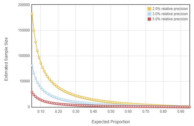
In the following figures, there is a drawing under two headings that represents the relationship between (Estimated Sample Size according to Expected Proportion). Fig. 3 under the title Estimated Sample Size according to Expected Proportion shows three curves, The first curve is in yellow color at 2% absolute precision. the second curve in blue color at 3% absolute precision. Finally, the third curve in red color at 5% absolute precision.
In the following figures, there is a drawing under two headings that represents the relationship between (Estimated Sample Size according to Expected Proportion). Fig. 4 under the title 95% level of confidence with sample sizes for (2, 3, and 5) three precision levels that show three curves, the first curve in yellow color at 2% relative precision. second curve in blue color at 3% relative precision. Finally, the third curve is in red color at 5% relative precision.
This plan refers to drawing a random sample from the final product amounting to (95) batteries and examining them. If the number of defectives is ( ), the sample is accepted and then the batch is accepted. But if the number of defective batteries is (
 ), the sample is rejected and a comprehensive examination is conducted for the remaining quantity (250-95) to isolate the not-good units and replace them with good ones, in addition to that, it was found that the average sample size for amputated sampling (
 ). And the probability of acceptance when the sampling plan (
 ) will be
  .
.
In this section, there are two tables and one figure showing the random sample values and Inspection results of the random sample which represent the control limits in Fig. 5 of the lot. Table 2 represents a sample from the data. The inspection processes are shown the Table 3.
|
|
|
|
|
|
|
|
1 | 0.01 | 26 | 0.10 | 51 | 0.02 | 76 | 0.03 |
2 | 0.04 | 27 | 0.00 | 52 | 0.02 | 77 | 0.06 |
3 | 0.04 | 28 | 0.01 | 53 | 0.01 | 78 | 0.02 |
4 | 0.03 | 29 | 0.01 | 54 | 0.03 | 79 | 0.02 |
5 | 0.03 | 30 | 0.01 | 55 | 0.03 | 80 | 0.05 |
6 | 0.03 | 31 | 0.01 | 56 | 0.05 | 81 | 0.05 |
7 | 0.04 | 32 | 0.02 | 57 | 0.03 | 82 | 0.02 |
8 | 0.05 | 33 | 0.02 | 58 | 0.04 | 83 | 0.09 |
9 | 0.04 | 34 | 0.02 | 59 | 0.02 | 84 | 0.05 |
10 | 0.04 | 35 | 0.04 | 60 | 0.11 | 85 | 0.06 |
11 | 0.01 | 36 | 0.00 | 61 | 0.04 | 86 | 0.04 |
12 | 0.01 | 37 | 0.00 | 62 | 0.08 | 87 | 0.02 |
13 | 0.05 | 38 | 0.06 | 63 | 0.05 | 88 | 0.05 |
14 | 0.01 | 39 | 0.02 | 64 | 0.03 | 89 | 0.05 |
15 | 0.08 | 40 | 0.03 | 65 | 0.04 | 90 | 0.03 |
16 | 0.02 | 41 | 0.05 | 66 | 0.02 | 91 | 0.01 |
17 | 0.08 | 42 | 0.06 | 67 | 0.02 | 92 | 0.03 |
18 | 0.04 | 43 | 0.00 | 68 | 0.03 | 93 | 0.03 |
19 | 0.05 | 44 | 0.02 | 69 | 0.07 | 94 | 0.07 |
20 | 0.02 | 45 | 0.06 | 70 | 0.01 | 95 | 0.01 |
21 | 0.03 | 46 | 0.04 | 71 | 0.00 | ||
22 | 0.04 | 47 | 0.01 | 72 | 0.02 | ||
23 | 0.02 | 48 | 0.03 | 73 | 0.01 | ||
24 | 0.01 | 49 | 0.03 | 74 | 0.09 | ||
25 | 0.05 | 50 | 0.02 | 75 | 0.03 |
The inspection processes with an (x-bar) chart will be:
| (15) |
| (16) |
| (17) |
| (18) |
| |
The inspection processes are shown the Table 3. The number of defective batteries is ( ), the sample is rejected. The remaining items (250-95 = 155) showed inspection.
Inspection result | Number | Percentage |
Defective | 75 | 79% |
Effective | 20 | 21% |
Total | 95 | 100% |
The rate of sample size is one of the important indicators when applying the sample test to the product instead of the comprehensive examination. The use of the tabular examination method leads to a reduction in the amount of examination and contributes to reaching special decisions when the units examined are perishable or expensive, the higher the percentage of defective(P)gives lower (ASN) and becomes unnecessary. The need to apply a scientific method in the process of determining the optimal sample size and the number of defective units accepted because of its importance in reducing the cost of the examination process, determining different sample sizes based on different values for the risk of the producer and the consumer, as this allows for comprehensive monitoring of the product.
Salman Hussien Omran, Beta-Deficient Estimators with Truncated Sampling Plan in Quality Control for the Auto Battery Industry