PID Control for Balancing Bike Model using Reaction Wheel

The-Ngoc-Tram Tran 1, Thanh-Viet Ho 2,*, , Huu-Loi Nguyen 3, Ngoc-Nam Le 4, Van-Phuc Tran 5, Quoc-Bao Tran 6, Pham-Phuong Mai 7, Ngoc-Duy Pham 8, Tien-Phat Bui 9, Thi-Hong-Lam Le 10

1, 2, 3, 4, 5, 6, 7, 8, 9, 10 Ho Chi Minh city University of Technology and Education (HCMUTE), Vietnam

Email: 1 21151175@student.hcmute.edu.vn, 2 21151492@student.hcmute.edu.vn, 3 19142112@student.hcmute.edu.vn,  

4 19142076@student.hcmute.edu.vn, 5 20147315@student.hcmute.edu.vn, 6 20145401@student.hcmute.edu.vn,  

7 20145586@student.hcmute.edu.vn, 8 20151262@student.hcmute.edu.vn, 9 20142240@student.hcmute.edu.vn,  

10 lamlth@hcmute.edu.vn 

*Corresponding Author

Abstract— Motorcycles or bicycles are known as unbalanced systems like the inverted pendulum model. Normally, we must use a handlebar to control the Motorcycles or bicycles. In this paper, the authors propose a PID controller for a balance bike using a reaction wheel. The authors formulated a mathematical model for the system and performed simulation testing using MATLAB to control it. Also, the simulation model of the balance bike system using a reaction wheel has been developed to assess the feasibility of building and controlling the system without relying on its mathematical model. The study will explicitly provide the performance of the PID algorithm in controlling a balanced bike using a reaction wheel.

Keywords— Motorcycle; Bicycle; PID; Control Balance; Reaction wheel

1. Introduction

Two-wheeled vehicles have been widely used in the market, because of their usefulness in work and life. In automatic technology, people aim to balance their vehicles automatically. Numerous products are being developed and utilized in everyday life. The reaction wheel is a device commonly used in satellites and other smaller spacecraft for attitude control [1]. The structure of the device is simple: a disc mounted on a shaft, usually powered by an electric motor. The output torque of the reaction wheel is related to the motor torque and the moment of inertia. There are many control algorithms such as PID [3], fuzzy [4], LQR [5], sliding mode [6], etc. are very popular in laboratories. They can be used as methods to be tested on this model.

Numerous studies have been conducted on balancing inverted pendulums using various control strategies such as LQR [7], Fuzzy [8]-[9], LQR-Fuzzy, Linear Control [10], and sliding mode control [11][12]. PID control, the most prevalent control technique in the industry, is an enhancement of a basic control method known as proportional control. Proportional control, in its standalone form, can augment the feedback system’s speed. The integral effect (I) enables the system to maintain a stable and consistent output signal as it nears the desired value. The derivative effect (D) observes the rate of change in system performance over time and adjusts accordingly. This derivative effect prevents systems from becoming unstable when proportional and integral gains are increased.

In this paper, the authors propose a PID controller for a “Balanced Bike using Reaction Wheel” (BBRW). This will help newcomers to research, understand, and control more easily and help engineers and researchers to design self-balancing bikes or motorbikes.

2. Research Method

1. Mathematical Model of BBRW

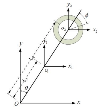
The Lagrange Method is a powerful approach to classical mechanics that provides an alternative perspective to the traditional Newtonian framework. It introduces the concept of the Lagrange, denoted as L, which combines a system's kinetic energy (K) and potential energy (V). By using generalized coordinates, the method derives Euler-Lagrange equations. Similar to the inverted pendulum [13][14], acrobot [15]. The system is based on the principle of an inverted pendulum with a reaction wheel, by skipping forces generated from steering and moving forward, a simplified dynamic model of the system can be derived using a Lagrange method for the BBRW system. Descarte's coordinate system was chosen in Fig. 1 [16][17] as follows:

1. Mathematical model of BBRW

Parameters of BBRW in Table 1 are recorded by actual measurement on the model. Tr is the input signal; the variables are θ,φ and Tr. φ and θ are output signals. Authors can find out the relationship among input/output signals referring to the algorithm [18]. Lagrange Method is obtained as [18]-[20] (1):

Where L is an equation that is determined by (2):

1. Parameters of BBRW

K is kinetic energy and V is potential energy; τi total force acting on the system;  are variables of the system.

From Fig. 1, the kinetic and potential energy of the system are defined by (3) and (4).

The system is around the equilibrium position [8]: sinθ ≈ θ; sin φ ≈ φ; cosφ ≈ cosθ ≈ 1.

From (3) and (4) the Lagrange equation is defined based on (2). Next, the calculating follows as (1), the mathematical equations of BBRW are described as:

 State Space equation is determined by (5) and (6) with the control signal as moment:

where: ,

To control the DC motor easily, the authors converted moment to voltage. The relationship between voltage and moment is described through [9]:

The parameters of the DC motor are shown in Table 2. The inductor value is much smaller than the return resistance value (), (8) can be written follow as: 

2. Parameters of DC motor

The relationship between motor speed and wheel speed is shown in (13):

where ωr is the angular velocity of the wheel.

From (8)-(12), the relationship between the applied voltage for the DC motor and the moment of the DC motor is:

From (7)-(13), mathematical equations of BBRW are.

where:

The state space variables are:

where:

The authors build an experimental model as in [https://www.thingiverse.com/thing:5887157] to examine our controller. The parameters were measured from the experimental model and referenced in [4]. The model’s specifications are illustrated in Table 3.

From formula (14) and the model’s specifications, we can determine matrices A and B as follows:

3. Parameters of the BBRW

Considering the control matrix , which has a non-zero determinant and rank (, we can conclude that the system is controllable with 4 state variables.

From (5), (6) and (13):

Using MATLAB to find the equations of , we obtain code in Fig. 2.

2. Math equation to calculate

 is q1_2dot and q2_2dot, the authors have found the equation that was computed using MATLAB:

2. PID Control for BBRW

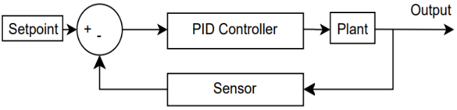
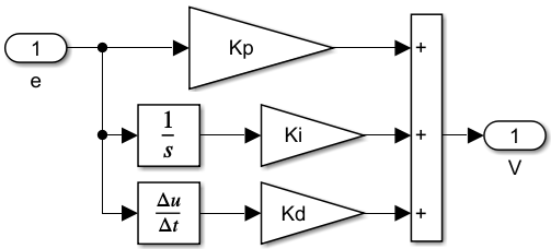
PID control (in Fig. 3) is a technique that combines three controllers: proportional, integral, and derivative. It can minimize the error to the lowest possible value, increasing the response speed, reducing overshoot, and limiting oscillation.

3. The structure of the PID controller

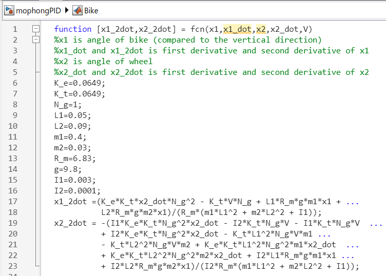
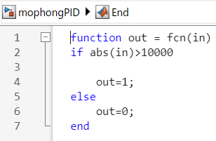
MATLAB simulation with system-measured parameters from the real-world model is shown in Fig. 4. The code of the description of the bike is shown in Fig. 5. “End block” in Fig. 4 guarantees the program not be stuck when the calculation is overloaded. The code of this block is shown in Fig. 6. The control block that describes the PID algorithm is shown in Fig. 7. 

4. Inside MATLAB Function block

5. System simulation diagram

6. Inside End block

7. Inside PID Controller block

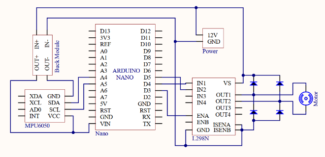
In addition to designing a system simulation on MATLAB/Simulink, the authors also built an experimental model controlled by a central CPU controller, Arduino Nano, and two sensors, including an MPU tilt sensor that measures the tilt angle of the vehicle body. Therefore, the continuous nonlinear system over time will be converted into a discrete system with a sampling time of 3ms.

3. Diagram and Flow chart

A wiring diagram is a visual representation of the electrical connections between electronic components. These components can be connected using cables or on a Printed Circuit Board (PCB). It is recommended that all components be connected to the Arduino Nano for optimal performance. The hardware connection diagram is presented in Fig. 8 and used on Altium software.

8. The writing diagram of BBRW

Based on the wiring diagram and the referenced model, below is the real-world model that the authors built in Fig. 9.

9. Real model of BBRW: (1): Body, (2): Reaction Wheel, (3): MPU sensor, (4): DC motor

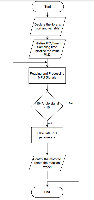
The flowchart algorithm was constructed to serve programming on the real-world model in Fig. 10.

10. Flowchart used in the control system

At the beginning, the program calls libraries and defines ports and variables. Then initialize the I2C, timer, determine the sampling time, and initialize the PID value. In the loop, the angular value of the MPU sensor is read continuously. Because the system operates stably from -10 to 10 degrees, the reaction wheel stops working if the reading angle exceeds the above value. If the read angle ranges from -10 to 10 degrees, calculate the PID parameter and output it to the reaction wheel control motor.

3. RESULT AND DISCUSSION

1. Simulation Results

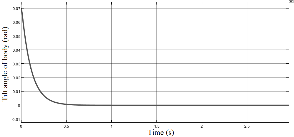
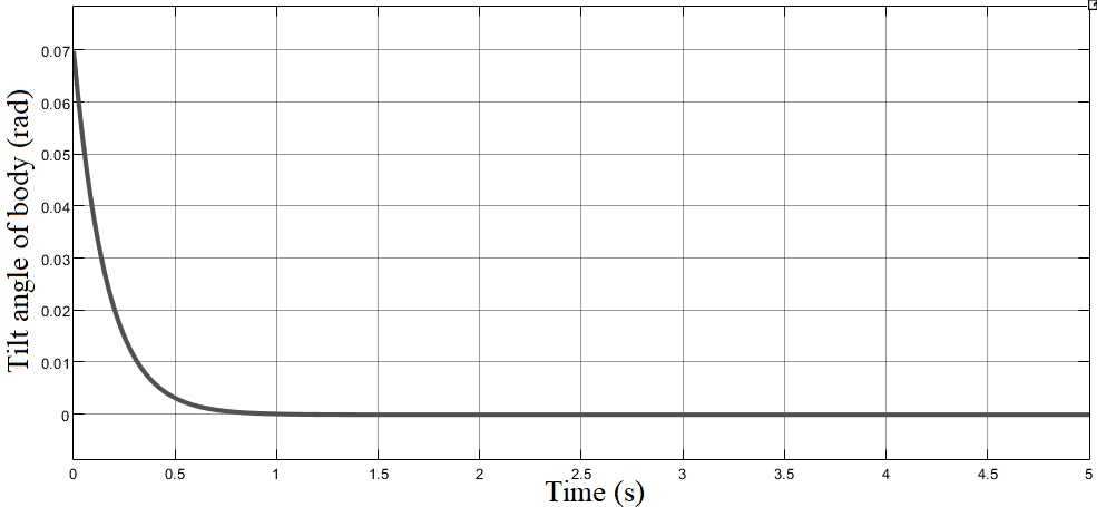
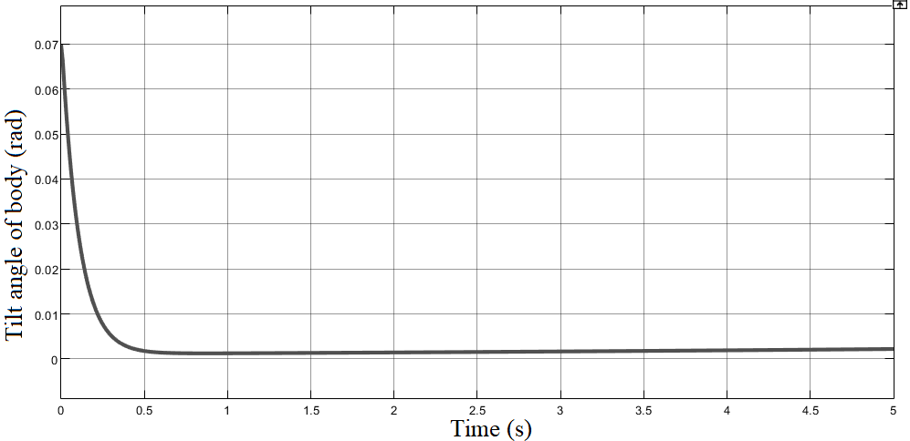
In the simulation section, BBRW was constructed based on the mathematical model, and the model’s parameters were measured from the real parameters of the balancing vehicle. The following is a balance survey of the vehicle when changing the P, I, and D parameters. Setpoint = 4-degrees for example. After the survey, the authors selected the following KP, KI, and KD parameters. Based on the graph, the settling time of the system can be inferred. Results are shown in Fig. 11 to Fig. 14. When Kp = 500, Ki = 150, Kd = 50; settling time is 0.5s. The system oscillates from 0.07 rad to the equilibrium position of 0 rad.

11. The tilt angle of the body under choosing PID parameters: Kp = 500, Ki = 150, Kd = 50

When Kp = 500, Ki = 150, Kd = 70, settling time is 0.75s. The system returns to equilibrium with longer periods.

12. The tilt angle of the body under choosing PID parameters: Kp = 500, Ki = 150, Kd = 70

When Kp = 500, Ki = 300, Kd = 50, settling time is 4s. The system overshoots a little and then gradually returns to equilibrium.

13. The tilt angle of the body under choosing PID parameters: Kp = 500, Ki = 300, Kd = 50

When Kp = 500, Ki = 75, Kd = 50, settling time is 0.6s. The system does not reach the equilibrium point, and when it is close to the equilibrium point, it becomes unstable.

14. The tilt angle of the body under choosing PID parameters: Kp = 500, Ki = 75, Kd = 50

Simulation observations:

• The system’s response signal is relatively good.
• If the absolute value of the input signal is the same, the response signal is the same.
• When changing the PID parameters, the system’s response signal changes.
• If Kd is increased, the settling time will increase. If Kd is decreased, the settling time will decrease, but if Kd is too low, the system may overshoot.

If Ki is increased, the steady-state error decreases, but if it is increased too much, the system may overshoot and become unstable. If Ki is decreased, the system cannot reach the equilibrium position and becomes unstable. The conclusion is that the model can be controlled.

2. Experimental Results

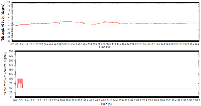
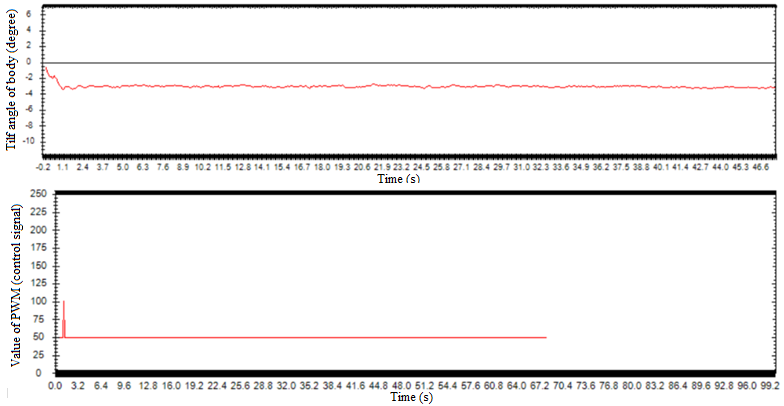
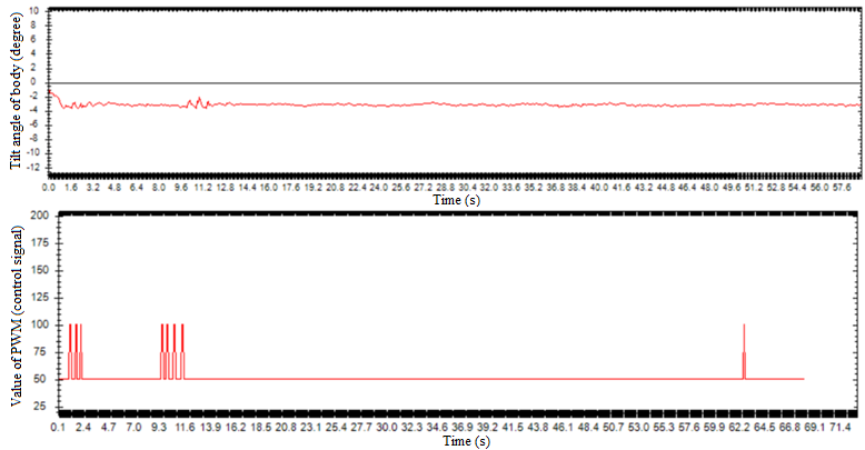
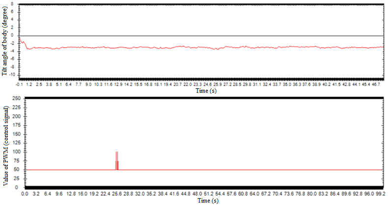
We applied the PID control algorithm to a real model. After surveying to change the parameters, the response results of the model when changing the P, I, and D parameters are presented from Fig. 15 to Fig. 18. Because there is the model error and sensor angle error, the setpoint angle for the model will be -1-degree. The first graph of each figure below is the actual angle signal of the model.

When Kp = 5, Ki = 30, Kd = 10, settling time is 55s. BBWR fluctuates steadily between 0 and -4 degrees, as shown in the figure below. The quality is maintained quite well, the control signal is stable.

15. The tilt angle (degree) (up figure) of the body and PWM control position (%) under choosing PID parameters: Kp=5, Ki=30, Kd=10

When Kp = 5, Ki = 5, Kd = 20, settling time is 0.6s. The system is stable within -4 degrees, due to the large wheels of the Bike, the system remains stable. Control quality is still quite good.

16. The tilt angle (degree) (up figure) of the body of the BBRW and PWM control position (%) under choosing PID parameters: Kp = 5, Ki = 5, Kd = 20

When Kp = 5, Ki = 5, Kd = 10, settling time is 12s. The system remains at -4 degrees but is unstable, causing poor control quality.

17. The tilt angle (degree) (up figure) of the body and PWM control position (%) under choosing PID parameters: Kp = 5, Ki = 5, Kd = 10

When Kp = 20, Ki = 5, Kd = 10, settling time is 2s. The system oscillates around the -4-degree position and the settling time increases. Control quality remains good.

18. Tilt angle (degree) (up figure) of the body of the BBRW and PWM control position (%) under choosing PID parameters: Kp = 20, Ki = 5, Kd = 10

Actual observation results:

• When increasing Kp, the system has overshoot but not significantly, the setup error and setup time decrease slightly. If the absolute value of the input signal is the same, the response signal is the same.
• When Ki increases, the setup error decreases but the system loses stability.
• When increasing Kd, the settling time decreases, and the system becomes more stable.

The P, I, and D parameters produced different results when adjusted with the real-world model. The reason for the difference in P, I, and D parameters between simulation and reality is measurement errors in the values and there are errors in the angle values of the MPU6050 sensor. Comparison between simulation and real-world model: In the simulation, BBRW was constructed based on a mathematical model, so it will affect the inclination angle of the vehicle with the inclination angle of the wheel. However, the model parameters are interdependent, and the inclination angle of the wheel is almost eliminated, so it may not be necessary to consider the inclination angle of the wheel.

4. Conclusion

PID controller is proposed by authors that
controlled BBRW stably through both simulation and
experiment. The MATLAB simulation produced good results, with the balancing vehicle reaching equilibrium at the desired settling time. BBRW has achieved balance in a real-world setting, but it has not yet been optimized due to model errors and suboptimal design. The model is still rudimentary and serves the purpose of learning to some extent. The MPU is still susceptible to errors and noise. The sensor still experiences signal loss due to vibration during robot motion. The robot still does not have the optimal operating status. It still oscillates and is unstable in some cases.

Acknowledgment

We would like to express our sincere thanks to the Ph.D. Van-Dong-Hai Nguyen (HCMUTE), who guided the research team and completed the project. The video of the model's operation is presented at the following YouTube link:  https://youtube.com/shorts/1i5u7g-tx7o?si=6J0aDS0pUwBE7hFJ

References

1. S. H. Miri et al., “Optimal Stabling of Attitude Maneuver for a Special Satellite with Reaction Wheel Actuators,” ASME 2010 10th Biennial Conference on Engineering Systems Design and Analysis, pp. 133-141, 2010, http://dx.doi.org/10.1115/ESDA2010-24383.
2. P.-L. Nguyen et al., “PID Controller for Balancing One-Wheeled Self-Balancing Robot,” Robotica & Management, vol. 27, no. 1, pp. 23-27, 2022, https://doi.org/10.24193/rm.2022.1.5.
3. C. B. Kadua and C.Y.Patilb, “Design and Implementation of Stable PID Controller for Interacting Level Control System,” Procedia Computer Science, vol. 79, pp. 737 – 746, 2016, http://dx.doi.org/10.1016/j.procs.2016.03.097.
4. V. Do Tran, M. T. Nguyen, V. T. Ngo, and T. Van Nguyen, “Experimental Fuzzy Control for Tower Crane,” Journal of Technical Education Science, vol. 68, pp. 36–47, 2022,  https://doi.org/10.54644/jte.68.2022.1121.
5. M. Q. Nguyen, T. K. Le, D. K. Bui, T. V. Le, and T. T. Nguyen, “Application of Genetic Algorithm in Optimizing LQR Control for Ball and Beam,” Robotica & Management, vol. 28, no. 2, pp. 48-54, 2023, https://doi.org/10.24193/rm.2023.2.9.

6. V. D. H. Nguyen, X. D. Huynh, M. T. Nguyen, I. C. Vladu, and M. Ivanescu, “Hierarchical sliding mode algorithm for athlete robot walking,” Journal of Robotics, vol. 2017, 2017, https://doi.org/10.1155/2017/6348980.
7. X. D. Huynh, T. D. Nguyen, D. T. Nguyen, D. B. Hoang, and M. H. Pham, “LQR Control for Double-Linked Rotary Inverted Pendulum: Simulation and Experiment,” Robotica & Management, vol. 27, no. 1, pp. 09-13, https://doi.org/10.24193/rm.2022.1.2.
8. Y. M. Yassin, A. El Mahallawy, and A. El-Sharkawi, “Real time prediction and correction of ADCS problems in LEO satellites using fuzzy logic. The Egyptian Journal of Remote Sensing and Space Science, vol. 20, no. 1, pp. 11-19, 2017, https://doi.org/10.1016/j.ejrs.2016.03.002.
9. Y. E. Bezci, V. T. Aghaei, B. E. Akbulut, D. Tan, T. Allahviranloo, U. Fernandez-Gamiz, and S. Noeiaghdam, “Classical and intelligent methods in model extraction and stabilization of a dual-axis reaction wheel pendulum: A comparative study,” Results in Engineering, vol. 16, p. 100685, 2022, https://doi.org/10.1016/j.rineng.2022.100685.
10. M. D. Vo, V. D. Nguyen, D. H. Huynh, T. N. Nguyen, M. D. Tran, and M. T. Vo, “Linear Control Schemes for Rotary Double Inverted Pendulum,” Robotica & Management, vol. 28, no. 1, pp. 59-67, https://doi.org/10.24193/rm.2023.1.8.

11. H. C. Tran, B. H.  Nguyen, Q. V. Nguyen, H. T. Quach, M. T. Nguyen, and M. P. Cu, “Simulation and Experiment of Sliding Control for Reaction Wheeled Inverted Pendulum,” Robotica & Management, vol. 25, no. 1, pp. 33-37, 2020, http://robotica-management.uem.ro/index.php?id=726&L=0.
12. M. A. Tofigh, M. J. Mahjoob, M. R. Hanachi, and M. Ayati, “Fractional sliding mode control for an autonomous two-wheeled vehicle equipped with an innovative gyroscopic actuator,” Robotics and Autonomous Systems, vol. 140, p. 103756, 2021, https://doi.org/10.1016/j.robot.2021.103756.
13. M. Olivares and P. Albertos, “Linear control of the flywheel inverted pendulum,” ISA transactions, vol. 53, no. 5, pp. 1396-1403, 2014, https://doi.org/10.1016/j.isatra.2013.12.030.
14. L. B. Prasad, B. Tyagi, and H. O. Gupta, “Optimal Control of Nonlinear Inverted Pendulum System Using PID Controller and LQR: Performance Analysis Without and With Disturbance Input,” Int. J. Autom. Comput, vol. 11, pp. 661–670, 2014, https://doi.org/10.1007/s11633-014-0818-1.
15. F. Xue, Z. Hou and H. Deng, "Balance control for an acrobot," 2011 Chinese Control and Decision Conference (CCDC), pp. 3426-3429, 2011, https://doi.org/10.1109/CCDC.2011.5968708.

16. K. Kanjanawanishkul, “LQR and MPC controller design and comparison for a stationary self-balancing bicycle robot with a reaction wheel,” Kybernetika, vol. 51, no. 1, pp. 173–191, 2015, http://dx.doi.org/10.14736/kyb-2015-1-0173.
17. D. K. Kim, H. Yoon, W. Y. Kang, Y. B. Kim, and H. T. Choi, “Development of a spherical reaction wheel actuator using electromagnetic induction,” Aerospace science and technology, vol. 39, pp. 86-94, 2014, https://doi.org/10.1016/j.ast.2014.09.004.
18. B. H. Nguyen, M. P. Cu, M. T. Nguyen, M. S. Tran, and H. C. Tran, “LQR AND FUZZY CONTROL FOR REACTION WHEEL INVERTED PENDULUM MODEL,” Robotica & Management, vol. 24, no. 1, 2019, http://robotica-management.uem.ro/index.php?id=704&L=0.
19. T.-T.-H. Le, “Input-Output Feedback Linearization Associates with Linear Quadratic Regulator for Stabilization Control of Furuta Pendulum System,” Robotica & Management, vol. 28, no. 1, pp. 28-35, 2023, https://doi.org/10.24193/rm.2023.1.4.
20. S. H. Chan, R. Khoshabeh, K. B. Gibson, P. E. Gill and T. Q. Nguyen, "An Augmented Lagrangian Method for Total Variation Video Restoration," in IEEE Transactions on Image Processing, vol. 20, no. 11, pp. 3097-3111, 2011, https://doi.org/10.1109/TIP.2011.2158229.