Journal of Fuzzy Systems and Control, Vol. 2, No 2, 2024 |
|
Adaptive Evaluation of LQR Control using Particle Swarm Optimization for Pendubot
Duc-Anh-Quan Nguyen 1, Luu-Quang-Thinh Nguyen 2*, Phong-Luu Nguyen 3, Duc-Quy Le 4, Phu-Thuan-An Lieu 5,
Quang-Buu Lam 6, Anh-Thu Tran 7, Tran-Tien Nguyen 8, Dinh-Luan Pham 9, Binh-Hau Nguyen 10
1, 2, 3, 4, 5, 6, 7, 8, 9 Ho Chi Minh City University of Technology and Education (HCMUTE), Vietnam
10 Posts and Telecommunications Institute of Technology, Vietnam
Email: 1 20151408@student.hcmute.edu.vn, 2 20151063@student.hcmute.edu.vn, 3 luunp@hcmute.edu.vn, 421151155@student.hcmute.edu.vn, 5 19142002@student.hcmute.edu.vn, 6 19142087@student.hcmute.edu.vn,
7 20124327@student.hcmute.edu.vn, 8 20151417@student.hcmute.edu.vn, 9 21151127@student.hcmute.edu.vn,
10 nguyenbinhhau@ptithcm.edu.vn
*Corresponding Author
Abstract—Pendubot is a classical system with high nonlinearity used in researching control algorithms. The Pendubot has a single input and multiple outputs (SIMO) and is under-actuated. In this paper, the focus is on studying the application of the Particle Swarm Optimization (PSO) algorithm to find optimal parameters for the LQR controller. The results obtained by the PSO algorithm will be compared when running with different parameters. Evaluations of the performance when applying the PSO algorithm to find optimal parameters will be drawn based on simulation results in Matlab/Simulink and experimental outcomes with various scenarios.
Keywords—Pendubot; Particle Swarm Optimization; LQR Control; SIMO System
Introduction
The Pendubot, along with under-actuated models in general, represents a nonlinear system with complex dynamical structures widely applied in technical control engineering research [1]-[3]. In numerous experiments, the simplified Pendubot model, in comparison to larger systems such as rockets or robots, serves as an ideal tool for mathematical development, control, and trajectory design. Research on these systems contributes significantly to the global field of control engineering.
In many studies, researchers have endeavored to design controllers with the aim of stabilizing the inverted pendulum system in the upright position using various methods. The Swing-up controller was developed to transition the pendulum from a stable equilibrium position (two links upright pointing downward) to an unstable equilibrium position, followed by switching to linear or nonlinear controllers for stabilization or tracking desired trajectories designed by the controller. In 2000, Spong et al. [4] designed a swing-up controller based on kinetic and potential energy, and there are also reports [5]-[7] on this controller applied to the Pendubot model. Balancing controllers have continuously evolved throughout the history of the Pendubot model, and nonlinear controllers applied to the Pendubot system have also been successively developed. For example, in the most recent development, Vu [8] developed a backstepping algorithm for this model, resulting in trajectory tracking with low error. In this paper, the authors focus on linear controllers. The first step in the paper is to model the Pendubot system. Then, the controllability of the system will be examined by linearizing the system at the operating point.; in [9], researchers studied the Input-Output Feedback Linearization Control, and in [10], the authors constructed an LQR controller with a Kalman filter. Based on [10], the authors built an LQR controller on both simulation and experiment by changing the input from torque to voltage, making the system more complex and more development-oriented.
With LQR control, selecting parameters to minimize errors and achieve stable operation is a challenging task. Therefore, the authors propose using the Particle Swarm Optimization (PSO) algorithm to optimize the parameters of the controller. PSO will assist in finding the values of the K matrix of the LQR controller. PSO was first introduced by Eberhart and Kennedy in 1995 [11]. This algorithm is based on the natural foraging behaviors of flocks of birds or schools of fish. Similar to genetic algorithm (GA), PSO is an intelligent algorithm based on the evolutionary experience of individuals in nature. In [12], Yuan et al. compared these two algorithms based on experiments, demonstrating that the PSO algorithm converges better but has poorer local minimum escape capabilities than GA. Numerous scientific publications on the PSO algorithm have been made throughout its development history. Publications [13]-[21] have made diverse developments and analyses of this intelligent method, with the flexibility of using the parameter w help the swarm balance between global and local search capabilities. In 2017, Wang et al. [22] published the most comprehensive and general analysis of the swarm and its parameters. In this paper, the authors will use the PSO algorithm to investigate the parameter search capabilities and compare different parameter sets based on the fitness function, thereby providing the most comprehensive overview of swarm optimization techniques. The contribution of the article will help research projects on PSO have additional reference materials as well as a premise for developing the use of PSO to find optimal parameters for nonlinear controllers such as Sliding Mode. Control - SMC or Backstepping controller.
Material and Method
Modeling of the pendubot system
Fig. 1 depicts the pendubot with two interconnected joints. This system has one input and multiple outputs (SIMO), which is a typical example of a highly nonlinear system. Joint one is directly linked and controlled  , while joint two is coupled to joint one through a connecting joint and equipped with an encoder to measure the angle
  . The mass of joint one (two) is denoted as, and the length of link one (two) is defined as
  , and the distance from the encoder axis to the center of mass of link one (two) is denoted as
  . The inertia moment is located at the center of mass of link one (two) and is defined as
  . We apply the Euler-Lagrange equation as (1).

- Dynamics of Pendubot

| (1) |
Where  is the position vector and
  is the velocity vector of the system,
  is the input of the control variable. The obtained dynamic equation of the system is expressed as follows:

| (2) |
where:
In addition,  is referred to as the inertia matrix,
  is referred to as the Coriolis matrix, and
  is referred to as the gravity matrix.
Since the actual input signal of the Pendubot system is the voltage supplied to the DC motor, the conversion of the first mathematical equation represented in (1) of the system to the new equation is expressed as follows:

| (3) |
The parameters used in this paper are defined as follows, as presented in Table 1.
- Parameters of system
Parameter | Description |

| Mass of link 1 ( ) ) |

| Mass of link 2 () |

| Length of arm’s center of mass ( ) ) |

| Length of pendulum’s center of mass () |

| Acceleration due to gravity ( ) ) |

| Coefficient of friction of the arm |

| Coefficient of friction of the pendulum rod |

| Inertia moment of link 1 ( ) ) |

| Inertia moment of link 2 () |

| DC motor resistance ( ) ) |

| Torsional moment constant |

| Angle of link 1 with respect to the horizontal axis ( ) ) |

| Angle of link 2 with respect to link 1 () |

| Angular velocity of the arm link ( ) ) |
| Angular velocity of the pendulum link () |

| Angular acceleration of the arm link () |

| Angular acceleration of the pendulum link () |
Analysis of System Controllability
Before designing control and filtering systems for any given linear system, it is necessary to assess the controllability and observability of the system. Starting from the nonlinear equations, linearization around the operating point of the system is performed. In this case, the control is chosen at the TOP position can be seen in Fig. 2.

- Top Position of the Pendubot
Analysis of System Controllability
Linear System:

| (4) |
When the system is stable, the state variables of the system will converge to zero:
The matrices A and B are obtained through linearization of the system around the operating point, resulting in:
Since the author team simulated the LQR controller on a discrete-time system, they utilized the c2d(A, B, sample time) command to convert it to a discrete-time system, where A and B are the linearization matrices and sample time is the system's sampling time.
The controllability matrix is given by:

| (5) |
Using the matrices A and B, we can assess the controllability of the system. If the rank of the controllability matrix, denoted as (5), is equal to the number of state variables, then we conclude that the system is controllable. Based on this, we can design a control system for the linearized system:
Therefore, based on the controllability matrix (5),  we can conclude that the system is controllable.
Design of the control system
The quality criteria can be expressed through the following fitness function:

| (6) |
The optimal control signal is designed as follows:

| (7) |
where K is the state feedback gain matrix determined by the formula:

| (8) |
P is the positive semi-definite solution of the algebraic Riccati equation:

| (9) |
The authors simulated the discrete-time system using MATLAB software. To obtain the control gain, they utilized the dlqr(A, B, Q, R) function, which allowed them to calculate the coefficient K for the control design, where Q and R are positive definite weighting matrices.
Particle Swarm Optimization (PSO) algorithm
Origin and background
PSO is a stochastic optimization technique based on swarm, which was proposed by Eberhart and Kennedy [11] is a computational optimization technique inspired by the social behavior of organisms, particularly birds flocking or fish schooling. In PSO, a population of potential solutions, called particles, move through the search space following the best-known positions found by individual particles and their neighbors. Each particle adjusts its velocity based on its own experience and that of neighboring particles, aiming to converge toward the optimal solution over successive iterations. PSO is commonly used to solve optimization problems where the search space is complex and may contain multiple local optima.
PSO is a swarm search process in which each individual, referred to as a particle, carries a potential solution to the optimization problem in a D-dimensional search space. It can remember both the swarm's and its own optimal positions, as well as velocities. In each generation, information about the particles is combined to adjust the velocity of each dimension, which is then used to calculate the particle's new position. The particles continuously change their states in the multidimensional search space until they reach equilibrium or an optimal state, or exceed computational limits. The only connection between different dimensions of the problem space is introduced through objective functions. Experimental evidence has shown that this algorithm is an effective optimization tool. Based on the analysis by the author group [22] in continuous space coordinates, the mathematical PSO can be described as follows. Assuming the swarm size is N, the position vector of each particle in D-dimensional space is  , velocity is
  , The optimal position of an individual (i.e., the optimal position experienced by the particle) is
  , and the swarm's optimal position (i.e., the best position experienced by any individual in the swarm's history) is represented as
  .
.

| (10) |
The global best position (GBest) is the best position among all individuals in the swarm. The updated formula for velocity and position proposed initially by Eberthart and Kennedy in 1995 [11] is presented as follows:

| (11) |
where : The velocity of the ith particle at iteration;
  The velocity of the ith particle at iteration;
  is a weight of local information;
  is a weight of local information;
  the best position of the particle;
  the best position of the swarm.
Parameters  in equation (11) are typically chosen based on experience. The function rand() generates random values from [0;1]. Equation (11) is divided into three components: the first component is the inertia term, the second is the cognitive term, and the third is the social term. These components are closely related to each other and play a crucial role in finding global optima. Without the first component, the algorithm is more suitable for global optimization when the initial population size is large. In this case, PSO is capable of performing local search when converging to the global best position.
As presented, Kennedy and colleagues [11] introduced a previous velocity component to allow particles to explore additional search space, enhancing their ability to search in new areas. The first component provides both local and global search capabilities for the problem, necessitating a balance between local and global exploration. In the late 1990s, Eberhart and Shi [19] proposed the addition of an inertia coefficient to balance local and global search. The proposed equation is presented below:

| (12) |
The inertia coefficient component, represented by the parameter  , with higher values allows particles to maintain inertia in exploring new regions of the search space. Optimizing and limiting the search region can adjust the coefficient to lower values, encouraging local exploitation of neighboring regions of the solution. Eberhart [19] analyzed the parameter solution through experimental validation, suggesting that w values should fall within the range [0.9, 1.2] to provide reasonable solutions.
In 2000, in an analysis published by Eberhart and Shi [17], comparing two inertia coefficients, Inertia Weight and Constriction Factors for the swarm algorithm, the authors introduced a new inertia coefficient added to the PSO algorithm to ensure convergence for the problem:

| (13) |
The Constriction Factor introduced into equation (13) is defined as follows:

| (14) |
In a paper published in 2007, Clecrk and Kennedy [23] after extensive survey-based research, discovered that when ϕ < 4, the swarm tends to slowly cluster around the best solution found in the search space and does not guarantee convergence. Conversely, when ϕ > 4, convergence is quickly assured. Typically, to ensure convergence using a constant ϕ = 4.1, values of χ ≈ 0.72984 and c1 = c2 = 2.05 are commonly used.
The method for updating the position of particles in PSO
Through each generation, the iteration repeats to determine the next position of the particle, governed by three components: The first component is the particle's previous velocity, the second component is the particle's best-known position compared to its current position, and the third component is the best-known position achieved in its history compared to its current position. By synthesizing these three vectors, we obtain the next position that the particle will achieve can be seen in Fig. 3 and Fig. 4.

- Flowchart of the PSO

- The process of updating particle position and velocity
Objective function
The objective function plays a crucial role in the process of searching for optimal parameters when using the PSO algorithm. It evaluates the adaptability of the optimized parameters to the problem being solved, and numerous proposals are related to assessing the fitness function. In [16], Yogesh Chaudhari proposed criteria for evaluating the fitness function to assess the adaptability of the parameters found using the genetic algorithm. Additionally, in another publication [24], the authors suggested fitness functions when the system has two or more problems to solve. Typically, there are many methods available to evaluate the fitness of the parameters. In this problem, the authors propose the Sum of Square error (SSE) method [25], presented below:

| (15) |
Where,  is The desired signal achieved,
  Is the outputs of the actual system, and
  Is the number of data points.
Applying the PSO algorithm to the pendubot system
PSO-LQR structure
The output of the pendulous model consists of four state variables: the angular deviation of link 1, the rate of change of angular deviation of link 1, the angular deviation of link 2, and the rate of change of angular deviation of link 2. To control using LQR, we need to find a matrix K to multiply with the four output state variables of the model and feedback to the pendubot model, the feedback signal is the stable control signal applied to the pendubot model. The structure of the PSO-LQR controller is illustrated in Fig 5.

- The pendulous system with LQR-PSO controller
In this problem, the authors evaluated the upper and lower bounds of the control matrix K. Therefore, instead of searching for matrices Q and R in the control, we decided to use PSO to directly search for the K matrix for control. This search is effective only if the upper and lower bounds of the parameters of the K matrix have been evaluated. However, in essence, for LQR, we still need to search for matrices Q and R. At that point, we can adjust the bounds of these parameters to optimize the problem. Matrix Q prioritizes convergence speed, while R minimizes energy consumption.
Selection of PSO Parameters
In this paper, the authors employed the position update method proposed by Shi and Eberhart in a paper in 2000 [17] and in the article [19], the authors applied PSO to find the control coefficients for the LQR controller. However, in this paper, the authors will compare the fitness of the parameters obtained in simulation and experimental results.
- In this paper, the selection of the inertia weight parameter w is crucial as it significantly influences both global and local search capabilities. Since the control parameters are evaluated and bounded within a certain range, the focus is on local search. Therefore, we choose w and gradually decrease it with each iteration by multiplying it by a damping factor
 , as outlined in a guideline by Heris [26]. This approach aims to concentrate the swarm’s search efforts locally around the vicinity of the optimal solution.
 - Selecting the coefficients and : In this study, the authors aim to achieve a balance between the cognitive and social components. Therefore, both coefficients and are set to 2.
- The coefficients
 are random coefficients with values ranging from 0 to 1.
 - The choice of velocity range to keep particles within the search space is typically limited to the range of
 . However, in this problem, we are uncertain about the maximum operating range of velocity, so we choose
  .
. - Choosing parameters for
 : Given that we have bounded the operating values, we select parameter ranges suitable for the system to enhance search efficiency and accuracy.
Simulation results and discussion
To assess the adaptability of the optimized parameters tuned by the PSO algorithm, we utilize MATLAB/SIMULINK software for simulation validation. The mathematical model is computed and identified to perfectly reflect the real-world model, enabling us to accurately evaluate the process using the PSO algorithm to assess adaptability through objective functions. In other words, based on equation (11), we compute the optimal function for the tuned parameters, where smaller parameters indicate higher adaptability and reliability, applied in simulations for visual assessment. Additionally, we integrate this LQR algorithm with the optimized parameters into the experimental model to conclude the smart swarm’s search capabilities. Simulations are conducted for 10 seconds, with a system sampling time of 0.02 seconds. The main parameters utilized in this paper are presented in Table 2. The simulation model of the pendubot system with the LQR controller is presented in Fig 6.
- The parameters used in the system
Parameter | Unit |
=0.11129 | (kg) |
=0.02929 | (kg) |
=0.13063 | (m) |
=0. | (m) |

| () |

| () |
=3.232 | () |
=0.06 | ( ) ) |
 =2.486e-07 =2.486e-07
| () |

- Pendubot simulation system
Where (1) gathers data extracted from the model's output. Here, the authors are concerned with minimizing the output error, evaluated in equation (11), during the initialization of the PSO algorithm. Block (3) represents the matrix K, found by the swarm, which is then multiplied by the output state variables to generate the control signal for the model.
PSO assists in searching for values of  . Therefore, the swarm parameters are selected in Table 3. Proceeding with the simulation using the following initial values:
 and
and  . The simulation results are presented in Fig 7, Fig 8, and Fig 9.

- The response of the output signal q1 for different parameters
- Parameters of the PSO algorithm
Parameter | Value |

| -100 |

| 0 |

| -50 |

| 0 |

| -100 |

| 0 |

| -50 |

| 0 |
MaxInteration | 50 |
Swarm Size | 200 |
w | 1 |
wdamp | 0.92 |
| 2.4 |
| 2.22 |

| 
|

| 
|

- The response of the output signal q2 for different parameters

- The response of the output signal for different parameters
The fitness function values are evaluated based on equation (11) as shown in the Table 4.
- The fitness function and coefficients are calculated based on the simulation
Parameter | 
| 
| 
| 
| Fitness value |

| -29 | -8 | -30 | -5 | 4.3407 |

| -35 | -5.95 | -34.0 | -3.6 | 3.146 |

| -42.8 | -8.22 | -40 | -5 | 3.0728 |
Based on the results of the K values obtained using the PSO algorithm, the authors utilized them for simulation and evaluation based on the fitness function in Table 4. It can be observed that for the obtained K values, the system exhibits the ability to control balance. We can see that for the obtained parameter sets, we can effectively control the pendulous model in the simulation. However, for a given set of parameters, we can evaluate which parameters are better than others. In Fig. 7 and Fig. 8, parameter sets with smaller fitness values tend to spike more, but they converge to 0 faster compared to parameter sets with larger fitness values. The control signals depicted in Fig. 9 also demonstrate that the system requires more energy to return to equilibrium sooner for parameter sets with larger fitness values.
Experimentation results
The Pendubot system is designed for the application of the researched algorithm, presented as follows. The model components are built based on the divided components as depicted in Fig. 10 and include:
- STM32F407 Discovery microcontroller.
- Nidec DC servo series F motor with 200 pulse encoder sensor.
- First arm of the system.
- Second arm of the system.
- Encoder sensor for the second arm with 600 pulses.
- IR2184 driver.
- 220 VAC - 24 VDC power supply converter.
- CP2102 USB UART converter circuit.
- 220 VAC power supply.

- Hardware completion of the Pendubot model
The experimental results based on the obtained parameters are shown in the Table 4. The fitness results of the parameters when applied in the experiment are presented in the Table 5.
- Evaluating the fitness function in the experiment based on the obtained parameters
Parameter |
|
|
|
| Fitness value |
| -29 | -8 | -30 | -5 | 22.037 |
| -35 | -5.95 | -34.0 | -3.6 | 20.941 |
| -42.8 | -8.22 | -40 | -5 | 5.9798 |
Based on Fig. 11 showing the graphs of three output parameters , Fig. 12 showing the graphs of three output parameters, and Fig. 13 showing the control input of the system, it can be observed that all three LQR control parameters help balance the system, with the state variables oscillating around the zero position. However, it is particularly noticeable that in the graph in Fig. 14, both state  variables oscillate closer to position 0 compared to the graphs in Fig. 15 and Fig. 16, indicating that evaluating the system's adaptability with the control parameters in Fig. 14 using the formula (11) reflects that the smaller the output errors, the smaller the fitness function value, hence the better performance of the controller.

- The output response of the q1 signals based on experimental data

- The output response of the q2 signals based on experimental data
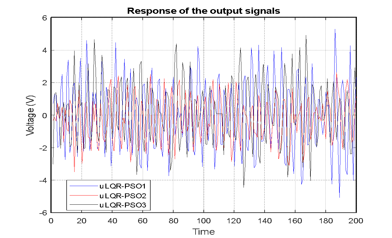
- The output response of the input signals based on experimental data
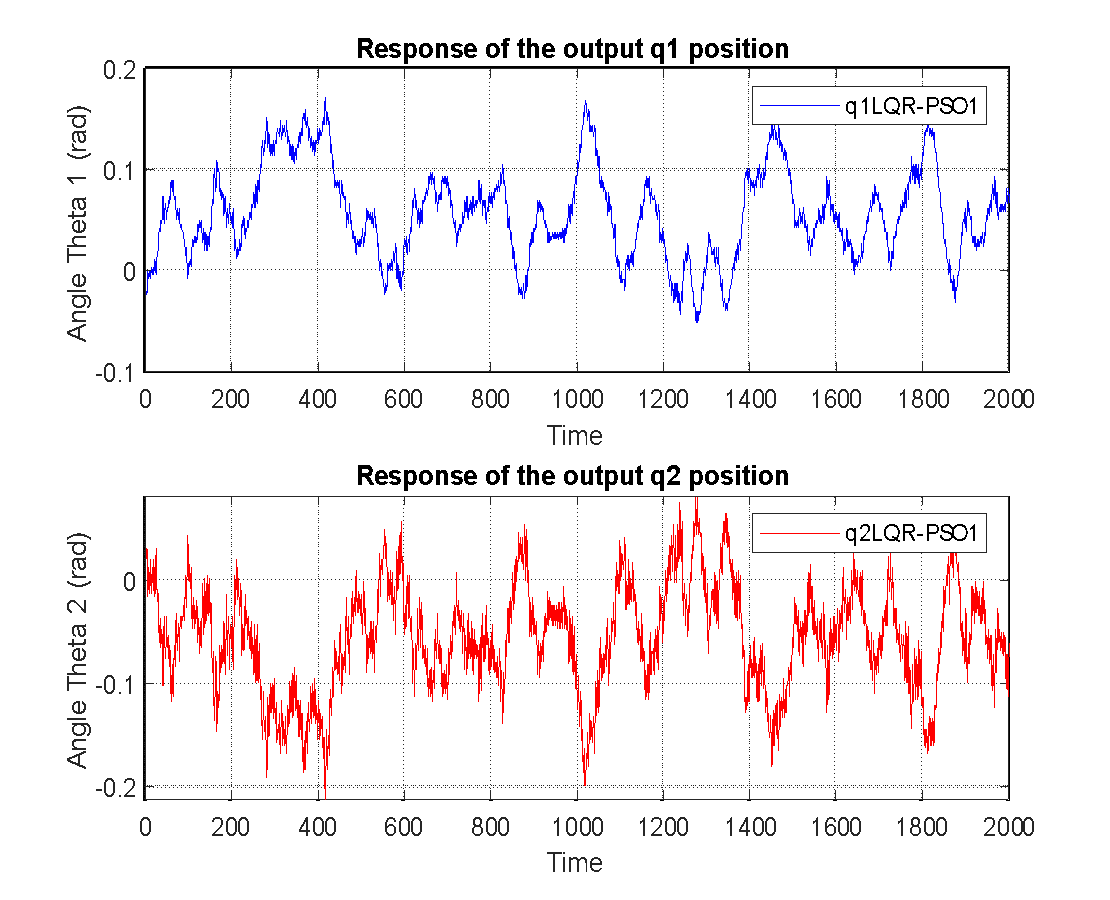
- The output of the two-state variables q1 and q2 from the LQR-PSO1 controller in the experiment

- The output of the two-state variables q1 and q2 from the LQR-PSO2 controller in the experiment

- The output of the two-state variables q1 and q2 from the LQR-PSO3 controller in the experiment
conclusion
In this paper, the authors investigated PSO, which is based on the concept of intelligent swarm behavior. Our goal was to utilize this intelligent algorithm to optimize the LQR controller parameters to the fullest extent possible. Therefore, we constructed an LQR controller and set objectives for the swarm to optimize these controller parameters. The results showed that through each parameter, based on the evaluation criteria of adaptability, we compared the responses in both simulation and experimentation. It can be concluded that the algorithm performs well, and the more optimized the fitness function, the better the response of the output according to each function. From the conclusions of the above article, it is possible to continue to develop the use of the PSO algorithm to find optimal parameters for nonlinear controllers.Video of the operation of the link is described in the link: https://www.youtube.com/watch?v=odQqVdEwSMc
References
- I. Fantoni and R. Lozano. Non-linear Control for Underactuated Mechanical Systems. Springer London. 2002. https://books.google.co.id/books?hl=id&lr=&id=Mk42P6AdrzgC.
- A. D. Luca, R. Mattone, and G. Oriolo, "Control of underactuated mechanical systems: application to the planar 2R robot," in Proceedings of 35th IEEE Conference on Decision and Control, vol. 2, pp. 1455-1460, 1996, https://doi.org/10.1109/CDC.1996.572718.
- M. W. Spong and D. Block, "The Pendubot: a mechatronic system for control research and education," Proceedings of 1995 34th IEEE Conference on Decision and Control, vol. 1 pp. 555-556, 1995, https://doi.org/10.1109/CDC.1995.478951.
- I. Fantoni, R. Lozano, and M. W. Spong, "Energy based control of the Pendubot," IEEE Transactions on Automatic Control, vol. 45, no. 4, pp. 725-729, 2000, https://doi.org/10.1109/9.847110.
- T. Albahkali, R. Mukherjee and T. Das, "Swing-Up Control of the Pendubot: An Impulse–Momentum Approach," in IEEE Transactions on Robotics, vol. 25, no. 4, pp. 975-982, 2009, https://doi.org/10.1109/TRO.2009.2022427.
- Xin, M. Kaneda, and O. K. I. T. Toshitaka, "THE SWING UP CONTROL FOR THE PENDUBOT BASED ON ENERGY CONTROL APPROACH," IFAC Proceedings Volumes, vol. 35, no. 1, pp. 461-466, 2002, https://doi.org/10.3182/20020721-6-ES-1901.00889.
- P. Ordaz, E. S. Espinoza, and F. Muñoz, "Research on Swing up Control Based on Energy for the Pendubot System," Journal of Dynamic Systems, Measurement, and Control, vol. 136, no. 4, p. 041018, 2014, https://doi.org/10.1115/1.4026658.
- C. Đặng Vũ et al., "Ứng dụng giải thuật Backstepping điều khiển ổn định hệ thống Pendubot: Mô phỏng và thực nghiệm," Tạp chí điện tử Khoa học và Công nghệ Giao thông, vol. 3, no. 4, pp. 27-37, 2023, https://doi.org/10.58845/jstt.utt.2023.vn.3.4.27-37.
- V. M. Tai et al., "Design of Input-Output Feedback Linearization Control for Rotary Inverted Pendulum System," Journal of Technical Education Science, vol. 17, no. 2, pp. 26-35, 04/28 2022, https://doi.org/10.54644/jte.69.2022.1120.
- H. A. Nguyen et al., "Application of LQG Control for Pendubot System," Journal of Fuzzy Systems and Control, vol. 2, no. 1, pp. 40-44, 2024, https://doi.org/10.59247/jfsc.v2i1.171.
- R. Eberhart and J. Kennedy, "A new optimizer using particle swarm theory," MHS'95. Proceedings of the Sixth International Symposium on Micro Machine and Human Science, pp. 39-43, 1995, https://doi.org/10.1109/MHS.1995.494215.
- Y. Duan, R. G. Harley and T. G. Habetler, "Comparison of Particle Swarm Optimization and Genetic Algorithm in the design of permanent magnet motors," 2009 IEEE 6th International Power Electronics and Motion Control Conference, pp. 822-825, 2009, https://doi.org/10.1109/CEC.2000.870279.
- S. Ghosal, R. Darbar, B. Neogi, A. Das, and D. N. Tibarewala, “Application of swarm intelligence computation techniques in PID controller tuning: A review,” In Proceedings of the International Conference on Information Systems Design and Intelligent Applications 2012 (INDIA 2012) held in Visakhapatnam, India, January 2012, pp. 195-208, 2012, https://doi.org/10.1007/978-3-642-27443-5_23.
- J. Barrera, O. Álvarez-Bajo, J. J. Flores, and C. Coello, "Limiting the Velocity in the Particle Swarm Optimization Algorithm," Computación y Sistemas, vol. 20, no. 4, pp. 635-645, 2016, https://doi.org/10.13053/CyS-20-4-2505.
- F. Chan and M. Tiwari. Swarm Intelligence: focus on ant and particle swarm optimization. BoD–Books on Demand. 2007. https://books.google.co.id/books?hl=id&lr=&id=-SmhDwAAQBAJ.
- A. Jayachitra, and R. Vinodha, “Genetic algorithm based PID controller tuning approach for continuous stirred tank reactor,” Advances in Artificial Intelligence, vol. 2014, pp. 9-9, 2015, https://doi.org/10.1155/2014/791230.
- R. C. Eberhart and Y. Shi, "Comparing inertia weights and constriction factors in particle swarm optimization," in Proceedings of the 2000 Congress on Evolutionary Computation. CEC00 (Cat. No.00TH8512), vol. 1, pp. 84-88, 2000, https://doi.org/10.1109/CEC.2000.870279.
- N. A. Selamat, F. S. Daud, H. I. Jaafar and N. H. Shamsudin, "Comparison of LQR and PID controller tuning using PSO for Coupled Tank System," 2015 IEEE 11th International Colloquium on Signal Processing & Its Applications (CSPA), pp. 46-51, 2015, https://doi.org/10.1109/CSPA.2015.7225616.
- Y. Shi and R. Eberhart, "A modified particle swarm optimizer," 1998 IEEE International Conference on Evolutionary Computation Proceedings. IEEE World Congress on Computational Intelligence (Cat. No.98TH8360), pp. 69-73, 1998, https://doi.org/10.1109/MHS.1995.494215.
- S. Yuan, D. Wang and X. Li, "The Application of PSO Algorithm on PenduBot Control," 2009 Fifth International Conference on Natural Computation, pp. 329-333, 2009, https://doi.org/10.1109/ICNC.2009.531.
- H. G. Kamil, O. T. Makki, and H. M. Umran, "Optimal tuning of a Linear Quadratic Regulator for Position Control using Particle Swarm Optimisation," IOP Conference Series: Materials Science and Engineering, vol. 671, no. 1, p. 012047, 2020, https://doi.org/10.1088/1757-899X/671/1/012047.
- D. Wang, D. Tan, and L. Liu, "Particle swarm optimization algorithm: an overview," Soft Computing, vol. 22, pp. 387-408, 2018, https://doi.org/10.1007/s00500-016-2474-6.
- D. Bratton and J. Kennedy, "Defining a Standard for Particle Swarm Optimization," 2007 IEEE Swarm Intelligence Symposium, pp. 120-127, 2007, https://doi.org/10.1109/SIS.2007.368035.
- Z. Bingül and O. Karahan, "A Fuzzy Logic Controller tuned with PSO for 2 DOF robot trajectory control," Expert Systems with Applications, vol. 38, no. 1, pp. 1017-1031, 2011, https://doi.org/10.1016/j.eswa.2010.07.131.
- J. Lu, W. Xie, and H. Zhou, "Combined fitness function based particle swarm optimization algorithm for system identification," Computers & Industrial Engineering, vol. 95, pp. 122-134, 2016, https://doi.org/10.1016/j.cie.2016.03.007.
- N. K. Jain, U. Nangia, and J. Jain, “A review of particle swarm optimization,” Journal of The Institution of Engineers (India): Series B, vol. 99, pp. 407-411, 2018, https://doi.org/10.1016/j.cherd.2018.03.031.
Duc-Anh-Quan Nguyen, Adaptive Evaluation of LQR Control using Particle Swarm Optimization for Pendubot








