Journal of Fuzzy Systems and Control, Vol. 2, No 2, 2024 |
|
A Survey of Experimental LQR for Cart and Pole
Dai-Phuc Hoang 1,*, Hoang-An Nguyen 2, Quang-Sang Pham 3, Huu-Chi Pham 4, Minh-Son Huynh 5, Duy-Phong Phan 6,
Nhut-Thanh Truong 7, Dinh-Phat Nguyen 8, Tran-Tu Uyen Nguyen 9, Hai-Thanh Nguyen 10
1, 2, 3, 4, 5, 6, 7, 8, 9 Ho Chi Minh City University of Technology and Education (HCMUTE), 01, Vo Van Ngan St., Linh Chieu ward, Thu Duc City, Ho Chi Minh City, Vietnam
10 Nguyen Huu Canh Technical and Economics Intermediate School, 500-502, Huynh Tan Phat St., Binh Thuan ward, District 7, Ho Chi Minh City, Vietnam
Email: 1 20145301@student.hcmute.edu.vn, 2 20151097@student.hcmute.edu.vn, 3 20151095@student.hcmute.edu.vn,
4 18142086@student.hcmute.edu.vn, 5 20145459@student.hcmute.edu.vn, 6 20145424@student.hcmute.edu.vn,
7 20145008@student.hcmute.edu.vn, 8 20145131@student.hcmute.edu.vn, 9 21145572@student.hcmute.edu.vn,
10 nguyenhaithanh@nhct.edu.vn
*Corresponding Author
Abstract—This study explores using an LQR control for a balancing model of the inverted pendulum (IP) on a cart and pole system at the equilibrium point. The approach starts by deriving the system's motion equations by Lagrangian method. Moreover, real-world experiments are conducted to validate the proposed control strategy, demonstrating its practical applicability and robustness specifically in the context of stabilizing IP systems on carts. Thence, this model can be a standard training model for laboratory in control theory.
Keywords—Cart and Pole; LQR Control; Inverted Pendulum; Optimal Control
Introduction
The story of IP serves as a quintessential example in the field of automatic control. Since the 1950s, it has evolved into one of the standard systems in control laboratories [1]. The diverse characteristics of IP, such as nonlinearity, instability, and single input-two output structure, render controlling an IP a challenging task. Furthermore, the dynamics of IP are fundamental for maintaining balance, applicable in scenarios such as rocket thruster control [2], walking [3][4], and wheeled mobile robot control [5][6], including recent innovations in personal transportation devices like self-balancing scooters [7].
The role of the IP paradigm in modern robotics extends to the development of bipedal robots, where researchers apply its principles to mimic the complex human gait, providing insights into the control of locomotion and balance [8]. As robotics systems become more sophisticated, the IP model continues to play a crucial role in the development of assistive exoskeletons designed to support and enhance human movement, especially for those with mobility impairments [9].
Within IP, there exist two equilibrium points, one stable position, and one unstable position. Consequently, controlling IP entails two objectives: swinging the pendulum to the upright position and maintaining this position. The primary challenge has been to maintain the upright position using a continuous feedback signal that can stabilize the pendulum around the unstable equilibrium, until recent advancements [10][11].
To address these control objectives, various control techniques have been applied to IP, including PID adaptive control [12], energy-based control [13][14], fuzzy control [15], neural network control [2], and quadratic linear regulator [11]-[16]. Additionally, a sliding mode control (SMC) approach has been employed to meet the necessary robustness performance [17]. SMC has been utilized for IP due to its established stability conditions and robustness [18]-[20].
While many control methods have demonstrated stable and accurate performance, employing LQR control is also a rational choice, particularly for optimizing control performance. Building upon the research topic of LQG Pendubot [21], the authors successfully refined a model of an IP on a cart using LQR control, achieving stable and precise positioning while effectively handling system disturbances and uncertainties.
MATERIAL AND METHOD
Physical Model without DC motor
The proposed physical model comprises a cart of mass  propelled by an applied force
  acting along the x-axis (see Error! Reference source not found.). A rod attached at the center of the cart is uniform and its mass is m. The rod is pivoted at one end, with its moment of inertia about the pivot point denoted as J. Positioned at a distance l from the pivot point is the center-of-mass of the rod. The cart and rod experience viscous friction, characterized by
  and
and  respectively. The input of the system is force , while the outputs are cart position
  and rod angle
  . Lagrange’s equations serve as a well-established and valuable tool for analyzing mechanical systems. The Lagrangian is defined as
  , where T represents the kinetic energy and
  denotes the potential energy of the system. With generalized coordinates x and θ, the Lagrange’s equations for the system can be expressed as:

| (1) |

| (2) |
The system's kinetic energy aggregates the kinetic energies of both cart and rod. Specifically, the cart's kinetic energy arises solely from its horizontal displacement, whereas the rod's kinetic energy stems from horizontal, vertical, and angular displacements. Notably, the horizontal and vertical center of mass positions of the rod are defined as  and
and  respectively. The total kinetic energy of the system is represented by:

| (3) |

| (4) |
With a homogeneous rod of length l, mass m, and pivoted at one end, a moment of inertia is calculated by [22] as:

| (5) |
The potential energy solely manifests as the potential energy of the pendulum, as the cart moves horizontally along the x-axis, rendering the potential energy of the cart null.

| (6) |
Lagrangian equation  of the system is presented as


| (7) |
Solutions to Lagrange’s equations (1) and (2) consist of nonlinear differential equations

| (8) |

| (9) |
Model with a DC motor
A DC motor featuring a constant field serves as a propellant for cart movement. The motor is activated through input voltage, denoted as  , to its armature terminal. Utilizing a wheel with a radius of r, the motor exerts a force to drive the cart, denoted as
  . With
  being formed by the rotor's moment of inertia
  , engine viscous friction
  , motor torque constant
  , pulley radius
  , and the armature current
  .
.

| (10) |
Whereas is calculated as follows, encompassing components such as motor supply voltage  , counter-electromotive force
  , and motor resistance
  :
:

| (11) |
Utilizing the Euler-Lagrange equation and employing MATLAB software enables the determination of the nonlinear equation of the system.

| (12) |

| (13) |
where  ;
;  ;
;  ;
;  . Parameters utilized in Fig. 1 are described according to the specifications provided in Table 1.

- Pendulum on a cart. Upward position (left). Downward position (right) [23]
- Parameters of the system
Parameter | Description |
| Mass of cart ( ) ) |

| Mass of pendulum () |

| Length of pendulum’s center of mass () |
| The radius of the pulley () |
| Engine viscous friction (N.s/m) |

| The coefficient of friction of the cart and track |

| The coefficient of friction of the pendulum rod |
| Rotor's moment of inertia ( ) ) |
| Rotor's armature resistance ( ) ) |

| Pendulum’s angle - theta ( ) ) |
| The vehicle's horizontal displacement. () |

| Acceleration due to gravity ( ) ) |
Examination of the system controllability
Before formulating control and filtering strategies for a linear system, it is imperative to evaluate the controllability and observability of the system. This typically involves linearizing nonlinear equations around the system's operating point. In the present scenario, the control is set to the TOP position  , as illustrated in Fig. 2.

- Top Position of the Cart-Pole System
The Linear System is presented as follows:

| (14) |
In a stable system, the state variables of the system will approach zero:

| (15) |
Matrices A and B are derived from the linearizing system around the operating point, yielding:
In order to simulate the LQR controller on a discrete-time system, we employed the c2d (A, B, sample time) command within the MATLAB application. This command facilitated the conversion of the controller to a discrete-time representation. Here, A and B represent linearization matrices, while sample time denotes the sampling time of the simulation. The presentation of the controllability matrix is stated as equation (16).

| (16) |
Utilizing matrices, A and B should the rank of the controllability matrix, designated as (16), match the number of state variables, it indicates the controllability of the system. This assessment allows for the design of a controller for a linearized system:
Hence, according to the controllability matrix (16), with  , we infer the controllability of the system.
SIMULATION
Proceeding with simulation using an identity matrix
To gauge the effectiveness of optimizing parameters using the LQR algorithm, we turn to MATLAB/SIMULINK software for simulation. Through meticulous mathematical modeling, we ensure an accurate reflection of real-world scenarios, enabling us to assess how well the LQR algorithm adapts via objective functions. Besides, we compute optimal functions for fine-tuned parameters, where smaller values denote superior adaptability and reliability, essential for intuitive simulations. Furthermore, we fuse this LQR algorithm with optimized parameters into our experimental model, shedding light on the intelligence swarm's quest capabilities. Simulations run for 10s, with a system sampling time of 0.02s. The main parameters are listed below:
- Parameters used in the system
Parameter | Unit |
= 0.19008 | (kg) |
= 0.084 | (kg) |
= 0.082 | (m) |
= 0.31258 | () |
= 0.00625 | (m) |
 = 0.096843 = 0.096843
| ( ) ) |
= 0.00039884 | () |
= 0.0058983 | ( ) ) |
= 1.4867 | () |
= 1.3663e-06 | () |
Fig. 3 depicts the simulation model with the LQR controller. Blocks (1), (2), and (3) collectively form an integrated system for analyzing and controlling the pendulum model. Block (1) functions as a data-gathering component, facilitating the comparison of different cases with varying K values. Block (2) simulates the pendulum model, producing outputs such as the cart position and pendulum angle. Finally, block (3) takes the output from block (2) as a control signal, simultaneously combining these signals into a virtual vector to be fed into matrix K, which is computed by employing matrices A and B to calculate for a linear quadratic state feedback regulator for the discrete-time state-space system.
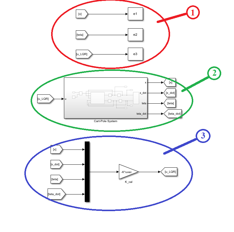
- Cart-Pole system
LQR algorithm aids in the determination of value for  . To identify appropriate K, one needs to initiate the search for parameters of Q and R matrices and commence experimentation starting with the identity matrix:
Upon reviewing Fig. 4, it demonstrates that control input (u) remains positive for the majority of the time, indicating that the system is supplying energy to the vehicle for motion. Control input gradually decreases over time, suggesting that the system is adjusting to maintain equilibrium.
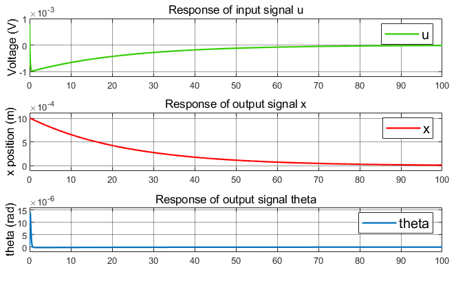
- The system's input and output with the identity matrix
The position of the vehicle (x) oscillates around the equilibrium position with an amplitude diminishing over time. This indicates system brings the vehicle back to its equilibrium position. Similarly, the pendulum angle (theta) also fluctuates around the equilibrium position, with its amplitude gradually diminishing over time. This illustrates the system's role in stabilizing the pendulum angle.
Optimizing control quality based on variations in Q1 and Q3
Based on the identity matrix, we adjusted the diagonal matrix with parameters named  and
and  , sequentially. The authorial team has selected four parameter adjustment scenarios for
  and
and  of matrix
  as follows:
- Case a:
 ,
,  , depicted by a green-colored line.
 - Case b:
 ,
,  , depicted by a blue-colored line.
 - Case c:
 ,
,  , depicted by a red-colored line.
 - Case d:
 ,
,  , depicted by a yellow-colored line.
Control signals are presented in Fig. 5 to Fig. 7.
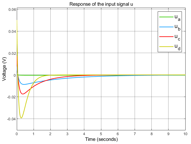
- Control signals u with Q variation
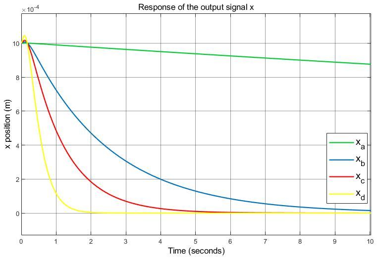
- Cart position signals (x) with Q variation
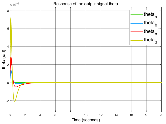
- Pendulum angle signals (theta) with Q variation
In case A, the longest settling time is observed, significantly surpassing that of the other three cases, as in Fig. 6, indicating the slowest attainment of the target position compared to other scenarios. However, overshoot is notably lower compared to the remaining three cases, readily observable in Fig. 7. Relatively high control energy consumption, denoted by u, is attributed to a substantially large settling time approaching zero, necessitating considerable energy to swiftly bring the system to its target position.
For case D, upon inspecting Fig. 5, shortest settling time and fastest approach to equilibrium position among all four cases are evident. Moreover, this case exhibits the highest overshoot among the four, as prominently illustrated in Fig. 6. Control energy consumption for case D in Fig. 5 is relatively low due to the short settling time, although the system is prone to instability owing to high overshoot. Upon scrutinizing Fig. 6 and Fig. 7 for the remaining two cases, it is apparent that systems are controllable due to acceptable settling time and overshoot levels.
From these observations, a tentative conclusion can be drawn that both  and
and  exert significant influences on the system. If surpasses , the control system tends to settle faster but with higher overshoot and energy consumption, potentially leading to instability. Conversely, a larger relative to results in a longer settling time, yet with reduced energy consumption, thus facilitating energy conservation.
Improving control quality by adjusting R
The research team chose 4 scenarios for adjusting the matrix , following the color conventions outlined in Section B above:
- Case a:

- Case b:

- Case c:

- Case d:

The results of collected control signals are as follows can be seen in Fig. 8:

- Control signals u with R variation
For both cases A and B, representing very small values of R, a remarkably rapid settling time is evident alongside significantly higher overshoot compared to the remaining two cases, prominently demonstrated in Fig. 10. Cases C and D, on the other hand, representing higher values of R, exhibit longer settling times and lower overshoots than the other two cases, indicating reduced energy consumption. Additionally, upon examining Fig. 9, it is noted that the settling time of case D is faster compared to case C, albeit with a slightly higher overshoot, which is insignificantly consequential. This serves as evidence that this scenario is the most stable, with energy consumption at an acceptable level. Furthermore, a general conclusion can be drawn regarding the impact of varying the R matrix on system stability, specifically that reducing R leads to decreased energy consumption, and vice versa.

- Cart position signals (x) with R variation
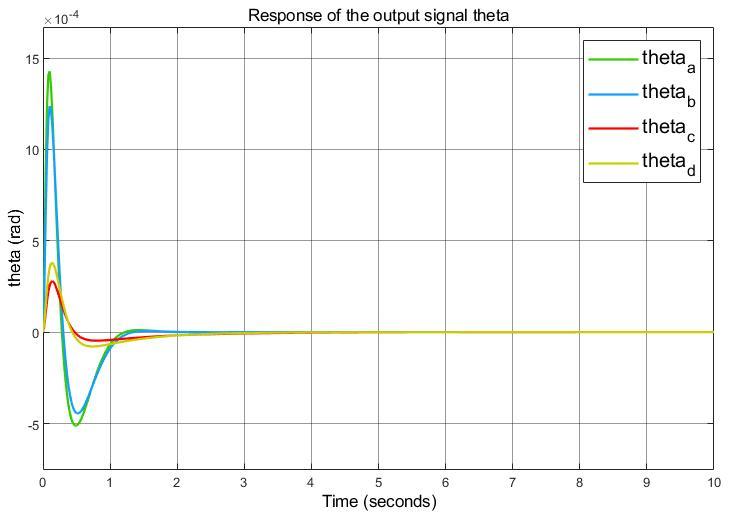
- Pendulum angle signals (theta) with R variation
EXPERIMENT
The cart-pole system has been meticulously engineered to implement the research algorithm. Model components are constructed according to segmented parts illustrated in Fig. 11, encompassing:
- H-Bridge MKS H3615NS.
- USB To TTL CH340G Converter Module Adapter.
- ST-LINK V2 STM8/STM32 Simulator.
- 220 VAC - 24 VDC power supply converter.
- STM32F407VET6 black board.
- Encoder sensor for the cart with 2500 pulses.
- Encoder sensor for the pendulum with 2500 pulses.
- Servo Motors NF5475.

- Finalization of the Cart-Pole Model's Hardware
We select to compare the three most stable operational scenarios as depicted in the simulation section, with three cases of varying R and Q selected as follows:
 and and 
|
Values of K calculated from selected Q and R matrices above are presented in Table 3. It illustrates experimental findings derived from acquired parameters:
- Matrices K are computed based on simulation.
Parameter | 
| 
| 
| 
|

| -50.2 | -53.1 | 69.8 | 6 |

| -23.4 | -47 | 61.2 | 5.3 |

| -16.7 | -45.6 | 59.3 | 5.2 |
Fig. 12 depicts plots of the system's three input parameters. Fig. 13 and Fig. 14 illustrate plots of three output parameters of x and theta, it is observed that all three LQR control parameters contribute to stabilizing the system, with state variables oscillating around position 0. However, in Fig. 16, both state variables x and theta oscillate closer to position 0 compared to plots in Fig. 15 and Fig. 17, indicating that evaluating the system's adaptability with control parameters in Fig. 16 with K matrix values reflecting the effectiveness of control based on carefully tuned Q and R matrices derived from the author's experience.

 signal input from experiments

 signal output from experiments

- Theta signal output
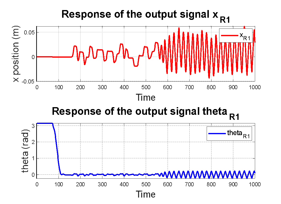
- and Theta states under LQR_1 controller's output

- and Theta states under LQR_2 controller's output
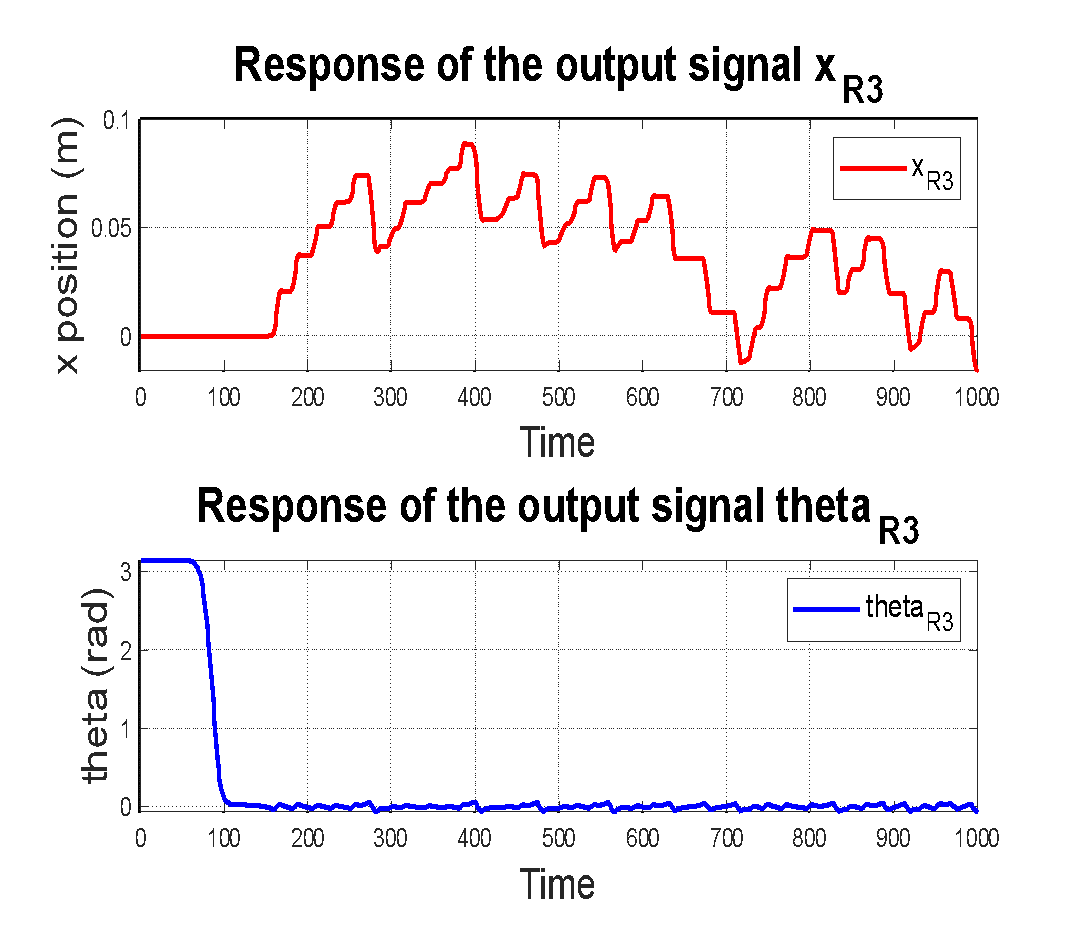
- and Theta states under LQR_3 controller's output
Thence, the investigation into individual components ,  , , and
  of weighting matrix Q has shed light on their distinct roles in shaping the behavior of the system. Specifically, component affects the stability of the cart's position. Component influences the cart's velocity. Component affects stability around the equilibrium position of the pendulum. Component impacts the pendulum's angular velocity and control effort. Additionally, the size of matrix R plays a crucial role; a large R slows down and stabilizes output voltage, while a small R tends to induce oscillations.
conclusion
This survey has provided a comprehensive analysis of the experimental LQR applied to the cart and pole system. One significant finding is the profound impact of matrices A and B, representing the state and control variables respectively, on the computation of the feedback gain matrix K. These matrices fundamentally define the dynamics of the system and directly influence the stability and performance of the LQR controller. By understanding the intricate interplay between these parameters, researchers can optimize the design of LQR controllers for cart and pole systems, balancing performance metrics such as stability, tracking accuracy, and energy efficiency. This deeper comprehension opens avenues for further exploration and refinement of control strategies, ultimately advancing the effectiveness and applicability of LQR techniques in real-world scenarios. Plus, the model in this survey is proved to be an experimental training system for the control laboratory.
ACKNOWLEDGEMENT
We want to give thanks to PhD. Van-Dong-Hai Nguyen due to his support in theory for this project. The video of operation of system is shown in link: https://www.youtube.com/watch?v=XUiZ87OrAqo
References
[1] K. J. Åström and K. Furuta, "Swinging Up a Pendulum by Energy Control *," IFAC Proceedings Volumes, vol. 29, pp. 1919-1924, 1996, https://doi.org/10.1016/S1474-6670(17)57951-3.
[2] C. W. Anderson, "Learning to control an inverted pendulum using neural networks," IEEE Control Systems Magazine, vol. 9, no. 3, pp. 31-37, 1989, https://doi.org/ 10.1109/37.24809.
[3] A. D. Kuo, "The six determinants of gait and the inverted pendulum analogy: A dynamic walking perspective," Human Movement Science, vol. 26, no. 4, pp. 617-656, 2007, https://doi.org/10.1016/j.humov.2007.04.003.
[4] J. H. Park and K. D. Kim, "Biped robot walking using gravity-compensated inverted pendulum mode and computed torque control," in Proceeding of IEEE International Conference on Robotics and Automation, vol. 4, pp. 3528-3533, 1998, https://doi.org/10.1109/ROBOT.1998.680985.
[5] J. SeongHee and T. Takayuki, "Wheeled inverted pendulum type assistant robot: inverted mobile, standing, and sitting motions," in 2007 IEEE/RSJ International Conference on Intelligent Robots and Systems, pp. 1932-1937, 2007, https://doi.org/10.1109/IROS.2007.4398961.
[6] N. Shiroma et al., "Cooperative behavior of a wheeled inverted pendulum for object transportation," in Proceedings of IEEE/RSJ International Conference on Intelligent Robots and Systems. IROS '96, vol. 2, pp. 396-401, 1996, https://doi.org/10.1109/IROS.1996.570801.
[7] M. Fadaei et al., "Data-Driven Control for Self-Balancing Two-Wheeled Scooter," in 10th RSI International Conference on Robotics and Mechatronics, pp. 7-10, 2002, https://doi.org/10.1109/ICRoM57054.2022.10025066.
[8] K. Wang et al., "Design and Control of SLIDER: An Ultra-lightweight, Knee-less, Low-cost Bipedal Walking Robot," in 2020 IEEE/RSJ International Conference on Intelligent Robots and Systems, pp. 3488-3495, 2024, https://doi.org/10.1109/IROS45743.2020.9341143.
[9] R. Kiran et al., "Impact of Exoskeleton Assistive Device for Physically Challenged and Elderly Patient for Rehabilitation Process," in 3rd International Conference on Innovative Mechanisms for Industry Applications, pp. 21-23, pp. 1499-1504, 2023, https://doi.org/10.1109/ICIMIA60377.2023.10426292.
[10] N. Muskinja and B. Tovornik, "Swinging up and stabilization of a real inverted pendulum," IEEE Transactions on Industrial Electronics, vol. 53, no. 2, pp. 631-639, 2006, https://doi.org/10.1109/TIE.2006.870667.
[11] B. Ata and R. Coban, "Artificial Bee Colony Algorithm Based Linear Quadratic Optimal Controller Design for a Nonlinear Inverted Pendulum," International Journal of Intelligent Systems and Applications in Engineering, vol. 3, no. 1, pp. 1-6, 2015, https://doi.org/10.18201/ijisae.87020.
[12] W.-D. Chang et al., "A self-tuning PID control for a class of nonlinear systems based on the Lyapunov approach," Journal of Process Control, vol. 12, no. 2, pp. 233-242, 2002, https://doi.org/10.1016/S0959-1524(01)00041-5.
[13] K. Yoshida, "Swing-up control of an inverted pendulum by energy-based methods," in Proceedings of the 1999 American Control Conference, vol. 6, pp. 4045-4047 vol.6, 1999, https://doi.org/10.1109/ACC.1999.786297.
[14] A. Siuka and M. Schöberl, "Applications of energy based control methods for the inverted pendulum on a cart," Robotics and Autonomous Systems, vol. 57, no. 10, pp. 1012-1017, 2009, https://doi.org/10.1016/j.robot.2009.07.016.
[15] L. X. Wang. Adaptive fuzzy systems and control: design and stability analysis. Prentice-Hall, Inc. 1994 https://dl.acm.org/doi/abs/10.5555/174457.
[16] A. Ghosh et al., "Robust proportional–integral–derivative compensation of an inverted cart–pendulum system: an experimental study," IET control theory & applications, vol. 6, no. 8, pp. 1145-1152, 2012, https://doi.org/10.1049/iet-cta.2011.0251.
[17] O. Boubaker, "The Inverted Pendulum Benchmark in Nonlinear Control Theory: A Survey," International Journal of Advanced Robotic Systems, vol. 10, no. 5, 2013, https://doi.org/10.5772/55058.
[18] L. Ji-Chang and K. Ya-Hui, "Decoupled fuzzy sliding-mode control," IEEE Transactions on Fuzzy Systems, vol. 6, no. 3, pp. 426-435, 1998, https://doi.org/10.1109/91.705510.
[19] N. Adhikary and C. Mahanta, "Integral backstepping sliding mode control for underactuated systems: Swing-up and stabilization of the Cart–Pendulum System," ISA Transactions, vol. 52, no. 6, pp. 870-880, 2013, https://doi.org/10.1016/j.isatra.2013.07.012.
[20] S. Mahjoub et al., "Second-order sliding mode approaches for the control of a class of underactuated systems," International Journal of Automation and Computing, vol. 12, pp. 134-141, 2015, https://doi.org/10.1007/s11633-015-0880-3.
[21] D.-A.-Q. Nguyen et al., "Application of LQG Control for Pendubot System," Journal of Fuzzy Systems and Control, vol. 2, no. 1, pp. 40-44, 2024, https://doi.org/10.59247/jfsc.v2i1.154.
[22] C. A. Manrique Escobar, C. M. Pappalardo, and D. Guida, "A parametric study of a deep reinforcement learning control system applied to the swing-up problem of the cart-pole," Applied Sciences, vol, 10, no. 24, p. 9013, 2020, https://doi.org/10.3390/app10249013.
[23] R. Saco, "Subspace Identification of an Inverted Pendulum on a Cart using State Variables Transformation," IFAC-PapersOnLine, vol. 52, no. 11, pp. 244-249, 2019. https://doi.org/10.1016/j.ifacol.2019.09.148.
Dai-Phuc Hoang, A Survey of Experimental LQR for Cart and Pole


