ANFIS-based LQR Control for Rotary Double Parallel Inverted Pendulum

Chi-Hung Nguyen 1, Van-Si Tran 2,*, Xuan-Hoang Nguyen 3, Quang-Bao Truong 4, Minh-Tuan Nguyen 5,

Nguyen-Phat Luong 6, Kha-Vy Ngo 7, Duc-Huy Nguyen 8, Thanh-Trung Nguyen 9, Thi-Thanh-Hoang Le 10

1, 2, 3, 4, 5, 6, 7, 8, 9, 10 Ho Chi Minh City University of Technology and Education (HCMUTE), Ho Chi Minh City, Vietnam

Email: 1 20151487@student.hcmute.edu.vn, 2 20151554@student.hcmute.edu.vn, 3 21151459@student.hcmute.edu.vn,

4 21151443@student.hcmute.edu.vn, 5 21151406@student.hcmute.edu.vn, 6 21151146@student.hcmute.edu.vn,

7 21151189@student.hcmute.edu.vn, 8 21151461@student.hcmute.edu.vn, 9 20145643@student.hcmute.edu.vn,

10 hoangltt@hcmute.edu.vn 

*Corresponding author

Abstract—This article explores two methodologies: Linear Quadratic Regulation (LQR) and the application of the Adaptive Neuro-Fuzzy Inference System (ANFIS) on the Rotary Double Inverted Pendulum in Parallel Type (PRDIP) model. This model belongs to a class of underactuated robots, representing a nonlinear system with a mechanically simplistic configuration yet exhibiting considerable nonlinearity. Therefore, ANFIS is utilized to learn the input-output data, responses, and feedback of LQR. The response of the system's output to both LQR and ANFIS is compared to demonstrate the effectiveness of ANFIS in learning from the principles of LQR. This demonstration is supported through three cases: one simulation case and two experimental cases. Both control strategies are applied to the PRDIP system at the zero and -π positions, where one pendulum remains upright, and the other descends to counteract oscillations. The study presents simulation and experimental results to evaluate the points above comprehensively.

Keywords—ANFIS; LQR; Rotary Double Inverted Pendulum in Parallel Type

1. Introduction

ANFIS is an integrated technique of Fuzzy Logic and Artificial Neural Networks. ANFIS combines the power of fuzzy inference in representing uncertain knowledge with the learning and self-adjustment capability of data [1]-[6]. ANFIS has been effectively applied in learning various control methods including Proportional-Integral-Derivative (PID), Linear Quadratic Regulator (LQR), and nonlinear control. These methods have been applied to Rotary Inverted Pendulum (RIP) [7][8] or pendulum systems [9], PID-based ANFIS control for Inverted Double Pendulum System [10], Adaptive Fuzzy Control of Two-Wheeled Balancing Vehicle [11]. Also, an ANFIS controller for the double double-inverted pendulum is operated [12]-[15]. A comparison of outcomes of ANFIS with LQR on these models is examined [16]. ANFIS is widely applied in automatic control systems such as robots, self-driving vehicles, and automated production systems, enhancing accuracy and performance [17]. It is utilized in predictive applications such as weather forecasting, price prediction, image classification, and signal analysis, leveraging its capability to learn from data and adapt flexibly [18]. ANFIS effectively processes and analyzes signals and images, finding applications in fields such as medicine, remote sensing, and information technology [19].

This article is facing LQR-Based ANFIS to PRDIP [20] an optimal control method at zero-π position, where one pendulum is upright while the other pendulum is downward-facing. PRDIP is considered an advance over previous models like RIP or Furuta pendulum, with improvements in mechanical design, including the addition of a parallel link to the existing arm [20]. Despite increased flexibility, PRDIP still faces challenges from nonlinear and unstable dynamics, particularly due to differences in pendulum lengths. Current research is concentrating on utilizing results from previously tested LQR control [20] to apply for re-learning ANFIS in controlling PRDIP.

ANFIS is a novel and effective algorithm for system control, particularly excelling over LQR in handling nonlinear systems through its ability to learn from real-world data. Unlike LQR, ANFIS does not require system linearity, making it applicable to more complex systems. It autonomously learns and adjusts parameters based on actual data, enhancing system adaptability to changes and environmental noise. The design and tuning of ANFIS can be more intuitive due to its automatic learning capability, reducing the burden on designers. By integrating fuzzy logic and neural network theory, ANFIS effectively manages systems with uncertainty and high noise levels. Its scalability allows the application of large and intricate systems, utilizing neural networks and fuzzy system structures. ANFIS learns directly from real data, enabling informed control decisions without the need for precise system modeling.

In summary, using ANFIS to learn from LQR outcomes and potentially replace LQR offers significant advantages in scenarios involving highly nonlinear, time-varying systems, or situations where accurate system modeling is challenging. ANFIS's ability to learn from real-world data and its flexible adjustment capabilities can substantially improve control performance across diverse conditions.

2. Mathematical Model of PRDIP

1. The undamentals of PRDIP

The physical structure includes two pendulums, an arm, two encoders, a DC motor, and an iron frame in Fig. 1, and the system's physical parameters are detailed in Table 1 [20]. Table 2 provides an overview of parameters relevant to PRDIP [20].

1. PRDIP model [20]

1. System parameters                                                                                                                                  

2. Values of system parameters

The mathematical equation of the system is calculated from the Lagrange function, denoted as.

The following is the Lagrange equation.

The kinetic energy equation

Velocities of the first and second pendulums are denoted as  respectively. Kinetic energy is re-written as

The system's potential energy is

Energy dissipation of PRDIP is contingent upon the frictional force

Lagrange equation is

        PRDIP employs a DC servo motor. The relationship between torque and voltage is described as

Values of the DC motor are shown in Table 3 [20].

3. Values of the motor's physical parameters

Dynamical equations of PRDIP are formulated in the form of state equations, presented as follows:

Dynamical equations of PRDIP are formulated in the form of state equations, presented as follows:

where

2. Linearized state equation

Consequently, linearization around the operational point (the upright position) becomes necessary for analysis and control.

The PRDIP's linearized state equation is as follows:

The matrices A and B are computed according to the following expressions:

where

Eigenvalues' positions are utilized to ascertain the stability of the system. The characteristic equation can be expressed in  where  are eigenvalues of . Matrices  and  are computed by substituting parameters of this system.

The open-loop poles of this system are determined in MATLAB using the command eig :

3. Building the controller

1. LQR controller

Consider a nonlinear system of the following form

is the system's state variable matrix; u is the control signal of the system.

Working point of is:

If u=0 then the system is balanced, and we can approximate the system in (1) to linear form

In there,

When the system works around this equilibrium position, we consider the system to be approximately a linear system so that designing a linear control algorithm is feasible. LQR control structure at the static working point of a linear system in (31) is shown in Fig. 2.

2. LQR controller structure

The selected control signal is

Computation of control matrix K typically involves solving complex Riccati equations. However, Matlab software simplifies this process by providing a lqr() command tool. Command to compute K is executed as follows:

In which, A and B are calculated in (3),  and  are weight matrices selected as follows.

With  and  are both positive constants

The LQR algorithm flow chart is shown in Fig. 3.

3. Flow chart of LQR controller

1. ANFIS Controller

Select an input and output data set for training consisting of  samples:

Step 1: Choose the learning rate , choose the maximum error .

Step 2: Booting up:

Assigning the error  

setting initial values for nonlinear parameters

Step 3: Estimating linear parameters using the least squares algorithm:

Step 4: Update nonlinear weights using gradient descent algorithm: With k=1:K

Calculate error:

Update error:

Calculate cumulative error:

Step 5: End a training cycle If E < , the learning process ends.

If E >= , assign E=0, and return to step 3 to start a new training cycle.

2. LQR-based Adaptive Neuro-Fuzzy Inference System (ANFIS) Controller        

The design methodology of LQR-based ANFIS is elucidated utilizing the algorithm delineated in parts A and B. ANFIS controller aims to emulate the functionality of a proficient LQR controller with a designated control matrix.

This matrix K is calculated according to (35) corresponding to the weight matrix Q, R found and optimized from the genetic algorithm (GA) for PRDIP with parameters in Table 1. Then, matrix K has the following values.

3. Building the data set

The dataset construction for ANFIS involves multiple inputs and outputs. It entails designing the optimal LQR map based on system parameters. The minimization of the cost function is treated as an optimization problem. Fig. 4 shows a program to create input and output files of the LQR algorithm. Fig. 5 shows the program used to collect input and output data of LQR to use for ANFIS learning.

4. The program simulates the system to create input and output data sets

5. Data collection program in MATLAB/Simulink

1. Determining the control parameters of ANFIS

The control parameters of ANFIS, including the number and type of membership functions, error tolerance, number of epochs, and learning method, are specified as follows:

To choose these parameters, we considered that our system is complex and difficult to control, so we chose these parameters based on the complexity of the system.

• The number of membership functions: 3
• Type of membership function: Trapmf
• Error tolerance: 0.386986
• Epochs’s number: 2
• Learning Format: Hybrid

1. ANFIS training

In ANFIS training, a structural block is formed by integrating parameters outlined in Part C to adapt to the collected dataset in Part D. Here, the dataset's "u" value serves as the output of the fuzzy inference system, while the remaining columns are treated as inputs. ANFIS training can be conveniently performed in MATLAB using the anfisedit command. The resulting .fis file serves as a state feedback controller for the designed system. Fig. 6 shows the interface of Toolbox ANFIS. We set corresponding parameters for learning to download data collected from the data collection program and start the learning process. Fig. 7 shows the interface of Toolbox ANFIS after completing learning and obtaining the data set for ANFIS. Error parameters of the learning process are shown.

6. ANFIS tool interface

7. Error value after training 2 epochs

Fig. 8 shows the program of the ANFIS system after learning the data of LQR. We use the FUZZY CONTROLER block to program ANFIS. Then, we see the results of ANFIS after learning LQR.

8. Program to simulate PRDIP system with LQR map based on ANFIS

4. Simulation results

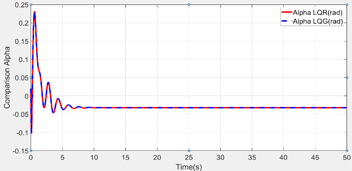
Fig. 9 shows the angular response of the arm bar. Initially, the arm deflection angle fluctuates strongly for the first 8 (s) with the largest amplitude of 0.22(rad), and after 10(s), the pendulum stabilizes around the working position, closely following the LQR response.

9. The output response of angle alpha

Fig. 10 shows the response to the angle of the first pendulum.  Initially, the arm deflection angle fluctuates strongly for the first 8 (s) with the largest amplitude of 0.08(rad), and after 10(s) pendulum stabilizes around the working position, closely following the LQR response.

10. Output response of angle theta1

Fig. 11 shows responses to the angle of the second pendulum.  Initially, the arm deflection angle fluctuates strongly for the first 10(s) with the largest amplitude of 3.43(rad), and after 13(s), the pendulum stabilizes around the working position, closely following the LQR response.

11. Output response of angle theta2

Fig. 12 shows the response to voltage. The system needs to supply a large amount of voltage for the first 15(s) to help two pendulum bars maintain balance, closely following the LQR response. The output response of ANFIS closely matching that of LQR indicates that ANFIS learns from LQR very effectively.

• Comment: The simulation results show that ANFIS has done a very good job in learning the output responses of LQR in Fig. 9, Fig. 10, Fig. 11, and Fig. 12. The output response of ANFIS is almost very close to LQR from which we can predict export using ANFIS controller instead of LQR controller on PRDIP system.

12. The response to voltage

5. Experimental

1. Experimental Mode

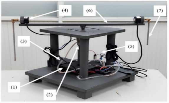
Fig. 13 is the actual model of the PRDIP system that we study in this article.

13. Realistic model

1. STM32F4007 microcontroller
2. Nisca NF5475 encoder motor
3. IR2184 H-bridge circuit
4. Encoder
5. USB to TLL CP2102 conversion circuit
6. Swing arm
7. Pendulum, Pendulum Lengths (Pendulum Short masses 0.059 kg and Pendulum Long masses 0.038 kg

1. Experimental Results

Case 1:

• Pendulum 1-Long is positioned upwards at the 0 radians mark, maintaining its balance.
• Pendulum 2-Short is positioned downwards at the -π radians mark, countering oscillation

Fig. 14 shows the angular response of the arm. For the orange response line, which represents the response of LQR, the oscillation amplitude of LQR is not large. In the range [40; 50] (s), amplitude oscillates strongly but then stabilizes at around 3 (rad). For the blue response line, which represents the response of ANFIS, the oscillation amplitude of ANFIS is very small, oscillating around 1 (rad), and the response is good. Therefore, the ANFIS controller learns to operate very well from the LQR.

14. The output response of angle alpha

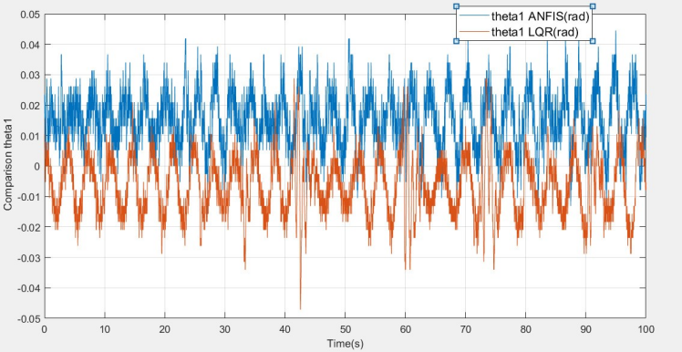
Fig. 15 shows the response to the angle of the first pendulum.  For the orange response line, which represents the response of LQR, the oscillation amplitude of LQR is small, in the range [-0.01; 0.02] (rad). Therefore, pendulum 1 responds well, balancing at position 0. For the blue response line, which represents a response of ANFIS, the oscillation amplitude of ANFIS is almost identical to the LQR controller, with a very good response. Thus, the ANFIS controller learns to operate very well from the LQR controller and can control pendulum 1 to balance at position 0.

15. The output response of angle theta1

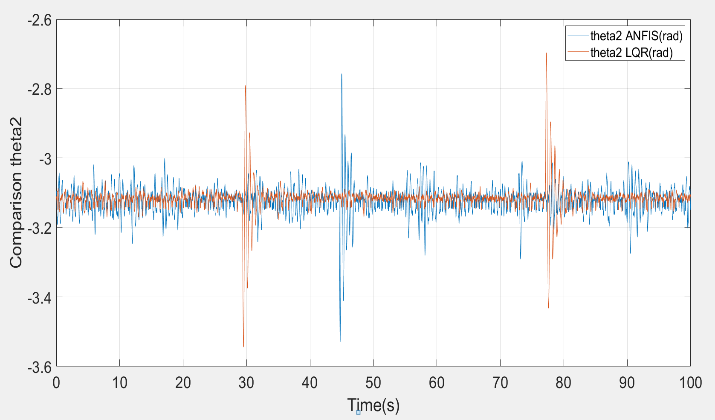
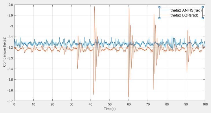
Fig. 16 shows the response to the angle of the second pendulum.  For the orange response line, which represents the response of LQR, the oscillation amplitude of LQR is very small around -3.14 (rad). At around 30(s) and 60(s), we deliberately apply a force to pendulum 2 in a downward direction to deviate it from the equilibrium position at -3.14, causing the response to deviate from the equilibrium position. So, pendulum 2 performs its function of reducing motion and immediately returning to the equilibrium position. For the blue response line, which represents the response of ANFIS, the oscillation amplitude of ANFIS is almost identical to the LQR controller, with a very good response. At around 45(s), similar to 30(s) and 60(s) intervals of the LQR controller, it performs well in reducing motion and immediately returning to the equilibrium position. Therefore, the ANFIS controller learns to operate very well from the LQR controller and can control pendulum 2 to balance downward at the equilibrium position of . The output response of ANFIS closely matches that of LQR. It indicates that ANFIS learns from LQR effectively.

16. The output response of angle theta2

Case 2:

• Pendulum 1-Short is positioned upwards at the 0 radians mark, maintaining its balance.
• Pendulum 2-Long is positioned downwards at the  radians mark, countering oscillation

Fig. 17 shows the angular response of the arm. The arm deflection angle fluctuates with an amplitude of 0.18(rad) within the range [-0.2;0.2]. For ANFIS control, the amplitude is 0.18 (rad) in the range [0.2; 0.6]. Therefore, the ANFIS controller can imitate the operation of the LQR controller which is very good.

17. The output response of angle alpha

Fig. 18 shows the response to the angle of the first pendulum. The deflection angle of the first pendulum will fluctuate within the range [-0.04;0.03]. For ANFIS control, it fluctuates within the range [-0.01; 0.04]. Therefore, the ANFIS controller has better performance imitation than the LQR controller.

18. The output response of angle theta1

Fig. 19 shows the response to the angle of the second pendulum. The deflection angle of the second pendulum will fluctuate within the range [-0.37;2.8]. For ANFIS control, fluctuating within the range [-3.2; -3.1]. For the angle of the second pendulum, the ANFIS controller has much better self-learning and adaptability than the LQR controller. It leads to better performance and greater stability in controlling complex systems, especially those requiring high precision such as LQR controllers. The output response of ANFIS closely matches that of LQR. It indicates that ANFIS learns from LQR very effectively.

• Comment: The responses of ANFIS in the test results above are very good, the output response of ANFIS closely follows the LQR and is in the control region so that the model runs best, with the above data we can see that the model is PRDIP runs very well. Therefore, ANFIS learns very well according to LQR and can replace the LQR controller to control the PRDIP system.

19. The output response of angle theta2

6. Conclusion

In this study, we propose to use MATLAB’s ANFIS toolbox to intelligently simulate a previously successful controller - LQR controller. This LQR-based ANFIS method has been shown to be successful in simulation and testing. Furthermore, this algorithm is also applied to the high-level SIMO system - PRDIP. From there, this study provides a reference for further research on ANFIS control for this type of model. In addition, the real-time model can be a hardware platform for training algorithm algorithms for students in the laboratory. Instead of using simple and popular controllers such as LQR, PID, etc., ANFIS will be used more in the future because ANFIS has many strengths such as ANFIS often giving high performance in controller applications. SIMO complexity, especially in linear and uncertain systems. This makes ANFIS an attractive option in many fields such as robotics, energy systems, and resource management. In this study, we also found the results of ANFIS-based LQR to be very good, not only as responsive as LQR but also better, thereby representing an important development and contribution to the following research on the PRDIP system and the results of this study are an important document that can be used for future system control studies.

ACKNOWLEDGEMENT

We want to give thanks to the PhD. Van-Dong-Hai Nguyen (HCMUTE) due to his support for us in operating the hardware. The operation of the system is shown in the link: https://www.youtube.com/watch?v=7A4pR9wB3dQ   

                                                  References

1. J. -S. R. Jang, "ANFIS: adaptive-network-based fuzzy inference system," in IEEE Transactions on Systems, Man, and Cybernetics, vol. 23, no. 3, pp. 665-685, 1993, https://doi.org/10.1109/21.256541.
2. K. Geetha and M. K. Hota, "Seismic Random Noise Suppression Using Optimal ANFIS as an Adaptive Self-Tuning Filter and Wavelet Thresholding," in IEEE Access, vol. 12, pp. 39578-39588, 2024, https://doi.org/10.1109/ACCESS.2024.3377143.
3. J. -S. R. Jang and Chuen-Tsai Sun, "Neuro-fuzzy modeling and control," in Proceedings of the IEEE, vol. 83, no. 3, pp. 378-406, 1995, https://doi.org/10.1109/5.364486.
4. M. D. Akmal et al., "Trajectory Tracking Control Design for Mobile Robot Using Interval Type-2 Fuzzy Logic," JFSC, vol. 2, no. 2, p. 67–73, 2024, https://doi.org/10.59247/jfsc.v2i2.200.
5. S. A. Aessa, E. H. Ali, S. W. Shneen, and L. H. Abood, "Adaptive Fuzzy Filter Technique for Mixed Noise Removing from Sonar Images Underwater," JFSC, vol. 2, no. 2, p. 45–49, 2024, https://doi.org/10.59247/jfsc.v2i2.176.

6. M.-Q. Nguyen, "Fuzzy Controller from Experts’ Rules for Middle Axis Ball and Beam," JFSC, vol. 1, no. 3, p. 80–84, 2023, https://doi.org/10.59247/jfsc.v1i3.94.
7. M. Abdullah, A. A. Amin, S. Iqbal, and K. Mahmood-ul-Hasan, “Swing up and stabilization control of rotary inverted pendulum based on energy balance, fuzzy logic, and LQR controllers,” Measurement and Control, vol. 54, no. 9-10, pp. 1356-1370, 2021, https://doi.org/10.1177/00202940211035406.  
8. Chawla, I. and Singla, A., "Real-Time Control of a Rotary Inverted Pendulum using Robust LQR-based ANFIS Controller," International Journal of Nonlinear Sciences and Numerical Simulation, vol. 19, no. 3-4, pp. 379-389, 2018, https://doi.org/10.1515/ijnsns-2017-0139.
9. Chawla et al., "Robust LQR Based ANFIS Control of x-z Inverted Pendulum," 2019 Amity International Conference on Artificial Intelligence (AICAI), pp. 818-823, 2019. https://doi.org/10.1109/AICAI.2019.8701333.
10. A. Kharola et al., "PID based ANFIS control of Inverted Double Pendulum System," 2022 Second International Conference on Next Generation Intelligent Systems (ICNGIS), pp. 1-5, 2022, https://doi.org/10.1109/54955.2022.10079899.

11. J. -Y. Chen et al., "Adaptive Fuzzy Control of Two-Wheeled Balancing Vehicle," 2011 First International Conference on Instrumentation, Measurement, Computer, Communication and Control, pp. 341-344, 2011, https://doi.org/10.1109/IMCCC.2011.92.  
12. Sheng Qiang et al., "ANFIS controller for the double inverted pendulum," IEEE International Conference on Industrial Informatics, Daejeon, pp. 475-480, 2008, https://doi.org/10.1109/INDIN.2008.4618147.
13. Y. Singh et al., "Design of ANFIS controller based on fusion function for the rotary inverted pendulum," International Conference on Advances in Power Conversion and Energy Technologies, pp. 1-5, 2012, https://doi.org/10.1109/APCET.2012.6302046.
14. Z. Qu et al., "Variable composition based adaptive fuzzy control of double inverted pendulum," Seventh International Conference on Fuzzy Systems and Knowledge Discovery, pp. 768-772, 2010, https://doi.org/10.1109/FSKD.2010.5569352.
15. A. Kharola and P. Patil, "Control of double inverted pendulum (DIP) using fuzzy hybrid adaptive neuro controller," 2014 IEEE International Conference on Computational Intelligence and Computing Research, pp. 1-7, 2014, https://doi.org/10.1109/ICCIC.2014.7238361.  

16. V. Mohan and N. Singh, "Performance comparison of LQR and ANFIS controller for stabilizing double inverted pendulum system," 2013 IEEE International Conference on Signal Processing, Computing and Control (ISPCC), pp. 1-6, 2013, https://doi.org/10.1109/ISPCC.2013.6663452.
17. HM Vu et al., "Design of hybrid fuzzy controller applied to snake robot," CTU J. Sci, vol. 55, no. 4, pp. 1-10, 2019, https://doi.org/10.22144/ctu.jvn.2019.090.
18. V. X. C. Del Rosario et al., "Weather Forecasting Rain Probability in Cebu Using ANFIS and Bayesian Network," 021 1st International Conference in Information and Computing Research, pp. 39-43, 2021, https://doi.org/10.1109/iCORE54267.2021.00026.
19. O. S. Vargas et al., "Adaptive Network-Based Fuzzy Inference System (ANFIS) Applied to Inverters: A Survey," in IEEE Transactions on Power Electronics, vol. 1, no. 39, pp. 869-884, 2023, https://doi.org/10.1109/TPEL.2023.3327014.
20. M. -T. Vo et al., "Linear Quadratic Regulators Optimal Control of Rotary Double Parallel Inverted Pendulum," 2023 International Conference on Control, Robotics and Informatics (ICCRI), pp. 14-18, 2023,  https://doi.org/10.1109/ICCRI58865.2023.00009.