Optimization of Linear Quadratic Regulator for Reaction Wheel Inverted Pendulum using Particle Swarm Optimization: Simulation and Experiment

Hau Nguyen Binh 1,*, Dat Tran Dinh 2, Anh Doan Cong3

1, 2, 3 Department II of Electrical Engineering, Posts and Telecommunications Institute of Technology, Ho Chi Minh,

Viet Nam

Email: 1 haunb@ptit.edu.vn, 2 dattd@ptit.edu.vn, 3anhdc@ptit.edu.vn

*Corresponding Author

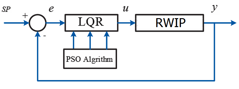
Abstract—This paper presents an optimization approach for the Linear Quadratic Regulator (LQR) applied to a Reaction Wheel Inverted Pendulum (RWIP) system, utilizing Particle Swarm Optimization (PSO). The study involves both simulation and real-world experimental verification. A mathematical model of the system is first developed using the Euler Lagrange method, and the LQR controller is designed to stabilize the highly nonlinear system, specifically a Single Input-Multiple Output (SIMO) system. PSO is employed to fine-tune the LQR parameters, optimizing performance metrics such as overshoot, settling time, and steady-state error. Simulation results, performed in MATLAB, are compared with experimental results obtained using an STM32F407 microcontroller-based hardware setup. PSO optimized LQR demonstrates significant improvements in stability and response time, outperforming standard optimization. The results confirm the efficiency of PSO in optimizing control systems for nonlinear dynamics, with potential applications in balancing robotics and self-stabilizing vehicles.

Keywords—Reaction Wheel Inverted Pendulum; Nonlinear; Upright Position; Linear Quadratic Regulator; Particle Swarm Optimization; Single Input-Multiple Output

1. Introduction

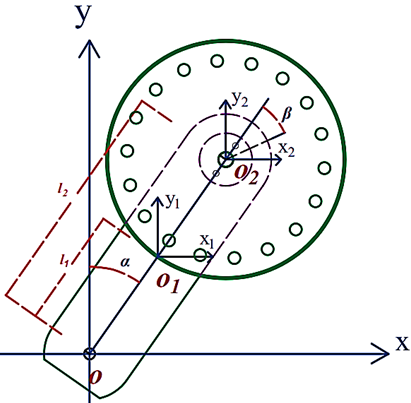
The RWIP system, often referred to as a gyroscopic balancing system, represents a quintessential example of a highly nonlinear dynamic system. This system consists of an inverted pendulum mounted on a reaction wheel. One end of the pendulum is attached to a free-rotating pivot, allowing unrestricted motion around the axis. The opposite end is connected to a motor, which drives the rotation of the reaction wheel. Consequently, the system features two primary output responses: the angular displacement of the pendulum () and the angular displacement of the reaction wheel ().

In the absence of a control mechanism, the pendulum would inevitably succumb to gravitational forces, leading to a loss of balance. The core challenge lies in continuously modulating the speed and direction of the reaction wheel to maintain the pendulum's upright position. This task mirrors the balancing required when riding a bicycle, necessitating constant and precise adjustments to prevent falling. The controller is responsible for generating control signals in the form of voltage inputs to the motor, which, in turn, produces the requisite torque to stabilize the system.

Comparable nonlinear systems, such as the rotary inverted pendulum [1][2], the ball-and-beam system [3], and the acrobot [4], also face significant challenges in achieving stable control. However, the complexity of the RWIP is amplified by the positioning of its actuator at the reaction wheel, located far from the base of the system. This configuration not only increases the difficulty of maintaining stability but also demands continuous and precise fine-tuning of control inputs. Furthermore, this system exhibits a SIMO structure, wherein a single control input - the voltage applied to the motor must regulate multiple outputs, specifically the pendulum angle () and the wheel angle ().

Over time, numerous control strategies have been explored for this system, including PID controllers [5], Fuzzy logic [6], and LQR [7]. Among these, the LQR stands out due to its capacity to effectively manage the complexities of nonlinear systems. In this study, we employ the LQR to optimize the control of the RWIP. The research methodology involves simulating the system's behavior under various conditions before validating the results through experimentation on a physical model. The authors developed the dynamic model with reference to the methodologies presented in [5]-[9]. Ultimately, the goal is to ensure the system maintains stability, even in the presence of external disturbances, by precisely controlling the wheel’s speed and direction.

2. DYNAMIC EQUATION OF MODEL SYSTEM

Based on the structure of the system placed on the Oxy coordinate plane, as shown in Fig. 1 and parameters where Table 1, the kinetic and potential energy of the system can be determined as in (1) and (2) (assuming approximations; ;  because the system is near the balance position):

The mathematical model of the RWIP system is formulated by applying the Lagrange method [7] as follows:

With L being the Lagrange equation defined by:

K is the kinetic energy and P is the potential energy of the system. is the sum of the constraint forces acting on the system.  are the coupling components that constitute the system.

The physical structure of the system is illustrated in Fig. 1 [7]:

1. Description of the structure of RWIP

1. Parameters of the System

The RWIP system can be extended to represent more complex systems, such as self-balancing bicycles and riderless motorcycles. In this context, the two primary control variables are the pendulum angle α and the wheel angle . Achieving precise control over the pendulum angle  ensures that the bicycle remains balanced. Similarly, controlling the wheel angle  effectively replicates the behavior of a rider leaning to maintain equilibrium. When the system is perfectly balanced, the rider would naturally return to an upright position. Therefore, successful manipulation of these two variables is crucial in demonstrating the viability of applying this system to future self-balancing bicycle models and autonomous motorcycles.

By calculating according to (3) and Table 1, we obtain the mathematical equations of the system as follows:

Establishing the state-space equations from (5) and (6), the mathematical representation of the system is described with the control signal as torque as follows:

Where:

Due to the conversion of the control signal from torque to voltage, the authors establish the relationship between the supplied voltage to the motor and the applied torque through the motor gear ratio as follows [7]:

2. Motor Parameters

With the inductance value being much smaller than the resistance value (L≪R), the voltage from (9) can be rewritten as follows:

The relationship between the motor speed and the wheel rotation speed is as follows:

Where ​ is the angular speed of the wheel.

From (8)-(12), the relationship between the supplied voltage to the motor and the applied torque can be determined as follows:

From (7) and (14), the mathematical model of the RWIP system with the control signal as voltage can be rewritten as follows:

Follow (15), with one input as the control signal (voltage U), and outputs consisting of two signals: the pendulum angle α and the wheel rotation angle β, represents a nonlinear SIMO system with one input and two outputs.

3. LQR  ALGORITHM

Due to the system that has a clear mathematical model, complete system parameters, and a specific, fixed operating point, LQR control algorithm is a common method. With its simple structure, ease of computation (thanks to MATLAB tools), and straightforward tuning based on weight matrices, the LQR controller is often recommended for balancing robot control. This is also the solution proposed for the system in this paper.

The system is described continuously over time as follows (assuming the system is approximated near the equilibrium position):

Where:

Adaptive Function is determined as (18):

Where: Q is matrix with n x n size, R is weighting matrix:

The control signal is feedback by LQR Algorithm as follow:

Where:

P is calculated by Riccati function as:

In all cases, we can set N=0 to simply calculate Riccati function. In order to find K matrix, authors use below command on Command Window of MATLAB Software:

Where matrices A, B and Q, R are determined from (20)-(22). Authors The authors have developed a Simulink model for the system.

2. Scheme of LQR controller for RWIP system

In this context, the matrix K is obtained by carefully selecting the weight matrices Q and R and incorporating the matrices Ad​ and Bd​ (derived from the discrete representation of the system at the equilibrium position). To compute the matrix K, the following command can be employed in MATLAB.

By analyzing the physical model depicted in Fig. 3, we can ascertain the system parameters as follows Table 3:

3. Physical model of the reaction wheel pendulum

4. Model in an uncontrolled state

3. Parameters of Real System

We can compute the matrices A and B at the equilibrium point, as given in (18). The resulting matrices are as follows:

Selecting the weighting matrices Q and R for an LQR controller is difficult using trial-and-error methods. Based on [10], a temporary set of values can be chosen to achieve an acceptable system response, with further tuning required for optimization.

Based on (25), (26), and Table 3, we can calculate the matrices A, B, and K.

However, the results were not favorable, as the system exhibited a slow response, particularly with the instability of the wheel speed Fig. 5. Therefore, we will next apply the PSO method to optimize the LQR coefficients.

5. LQR response corresponding to multiple selected Q and R matrices

4. PSO ALGORITHM

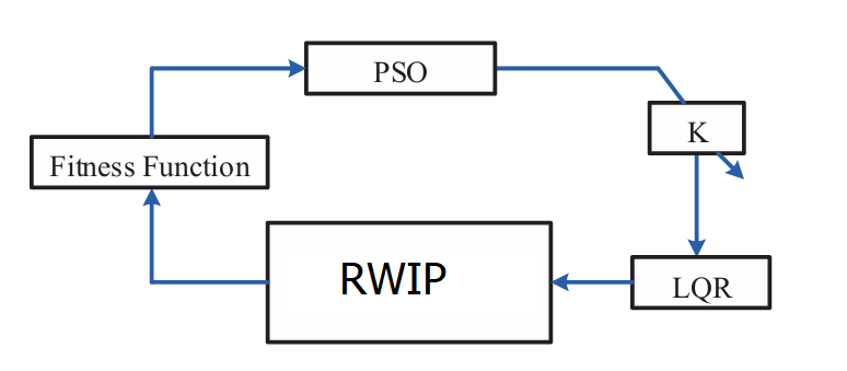
As shown in Fig. 5, identifying suitable matrix parameters Q and R poses significant challenges. Therefore, based on (21), we can directly optimize the parameter matrix K, which implicitly optimizes matrices Q and R as well. There are various methods for optimizing LQR, such as Sequential Quadratic Programming and Genetic Algorithm, however, this paper focuses on employing the PSO algorithm to determine the optimal values for matrix K, thereby inherently optimizing the LQR.

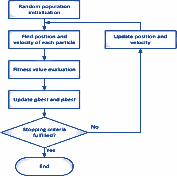
PSO is an evolutionary algorithm developed in 1995 by Kennedy and Eberhart [11]. The algorithm is inspired by the motion of swarms or flocks of animals, such as birds and fish. PSO mimics individual behavior in a swarm to enhance species survival and solves optimization problems through cooperation and competition among individuals over iterations. The algorithm maintains a global search strategy across the entire swarm while avoiding complex operations.

Due to its straightforward definition, ease of implementation, strong convergence, and robustness, PSO is appealing for addressing nonlinear problems. Numerous research studies have proposed applications of PSO in various control systems, including a linear state feedback controller based on the RWIP model. Comparisons of accuracy and computational efficiency between two evolutionary algorithms, GA and PSO, were investigated in references [11]-[16]. These studies demonstrate that PSO can achieve optimal results more quickly than GA.

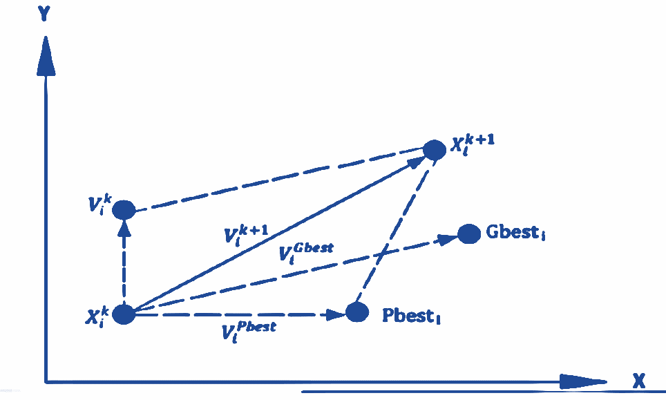
In a PSO system, each particle within the swarm adjusts its position by exploring various locations in the search space, ultimately converging on the best possible position. The concept of how PSO updates the search points is illustrated in Fig. 6 [13]. Each particle in the swarm is guided by its own best-known position and the best-known positions of the swarm as a whole, continuously refining its path until it reaches an optimal solution. This dynamic approach enables PSO to efficiently traverse the search space, making it a powerful tool for solving complex optimization problems.

6.  PSO vectorial notation

Where:

•  : Position of particle i at generation k.
• : Position of particle I at generation k+1.
• : Velocity of particle i at generation k.
• : Velocity of particle i at generation k+1.
• : Velocity towards the particle's
• personal best (Pbest).
• : Velocity towards the global best (Gbest).
•  The best-known position of particle i.
• : The best-known position of the entire swarm.

Due to clarify the concept of the PSO algorithm, let's consider the following example: imagine a flock of birds searching for food in a specific area. No bird knows the exact location of the food; however, they are aware of the distance to the food after each round of searching. The question arises: what is the best strategy to locate the food? The simple answer is to follow the birds that are closest to the food. PSO is inspired by this scenario and uses it to solve optimization problems.

In this context, each potential solution is referred to as a "particle." Within the framework of reaction wheel systems, these particles represent different configurations or control signals that can be applied to optimize system performance. Each configuration has an adaptive value assessed by a fitness function and possesses a velocity to direct its search for optimal solutions. The configurations explore the problem space by following those with the best current conditions.

PSO begins with a randomly initialized group of configurations and then seeks the optimal solution by updating through generations. In each generation, each configuration is updated based on two values: the first value, known as Pbest, is the adaptive value of the best configuration in the current generation. The second value, termed Gbest, represents the best solution that neighboring configurations have achieved up to the present time, or the adaptive value of the best configuration across all previous generations. In other words, each configuration in the system updates its position according to its own best position and the best positions of other configurations in the system as of the current time. The updating process for the configurations is based on the following two equations:

Where:

• n: The number of elements in the group.
• d: The dimension of the space.
• k: The number of iterations.
• v(k)i, m: The velocity of the ith node at generation k.
• w: The inertia weight.
• C1, C2: The acceleration coefficients.
• Rand (): A random number within the size of the group.
• x(k)i, m: The position of the ith node at generation k.
• Pbest i: The best location of the ith node.
• Gbest i: The best location of the node in the network.

According to [11]-[16], the operation of the PSO algorithm is illustrated in Fig. 7.

7. Flowchart of the PSO Algorithm

We initially reconstruct the optimal control model using PSO for the LQR system of the RWIP as follows Fig. 8, Fig. 9, and Fig. 10:

8. Diagram LQR controller for RWIP

9. Block diagram of PSO based LQR on inverted pendulum system

10. Simulation of the RWIP system for the PSO Algorithm

The simulation system for identifying the matrix K parameters is established based on (15), (21), and (24). The system's structure is illustrated in Fig. 11. The selection of initial PSO method parameters and identification process is described as follows:

• n = 5-100: Population size, representing the number of potential solutions being evaluated.
• bird_step(m) = 5-100: Maximum number of iterations allowed, which ensures sufficient exploration of the solution space (bird_step ≥ n).
• dim = 4: Dimensionality of the problem, corresponding to the four feedback gains (K1, K2, K3, K4).
• c2 = 1.2: Cognitive acceleration coefficient, guiding particles towards the global best.
• c1 = 0.12: Social acceleration coefficient, encouraging exploration of the particle's personal best position.

These parameter values are selected to balance convergence speed and the accuracy of the solution. The optimization targets identifying the optimal feedback gains for the LQR controller, specifically tailored for the RWIP system, ensuring efficient and stable control.

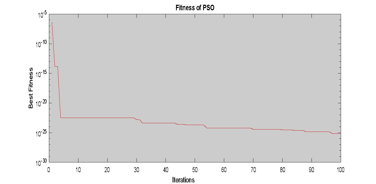
First, the population is initialized with a matrix of size n×m =5×5. The resulting outcomes are a shown in Fig.11, yielding an objective function value of J5x5=7.7391.10−19 and corresponding gain matrix k=1.0.103. [ 0.135 −1.331 0.052 0.169].

Next, for the matrix 10×10, the results are shown in Fig. 12, yielding an objective function value of J10x10​=1.8668.10−24 and corresponding gain matrix k= [−590.5414 −592.3087 60.8901 172.4309].

Subsequently, testing with a 50×50 population yielded the results shown in Fig. 13, with an objective function value of J50x50​ = 2.1506.10−26 and gain matrix k=1.0.103. [ −0.0769 −2.7523 0.2421 0.7964].

11. PSO with matrix 5x5

12. PSO with matrix 10x10

13. PSO with matrix 50x50

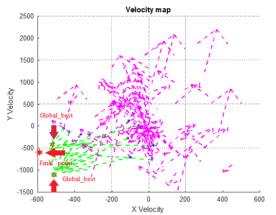
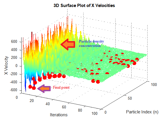
From the results of the 5×5, 10×10, and 50×50 populations shown in Fig. 12 and Fig. 13, we observe that the particle swarms tend to concentrate their search around the optimal points. Moreover, larger population sizes lead to increased speed and accuracy, as demonstrated by the objective function values: J5x5<J10x10<J50x50.

We initialize the PSO with a swarm size of 100x100 to obtain results for comparison with the selected LQR (26):

14. Graph of the J function for PSO 100x100

15. 3D map of velocity with swamp 100x100

16. PSO with matrix 100x100

From Fig. 14, Fig. 15, and Fig. 16, we can easily observe the collective behavior of the particles (birds) in the swarm. Once a particle discovers a point with favorable properties, the entire swarm quickly converges to search within that area. This approach is advantageous compared to the scattered search and multiple subdivisions utilized in Genetic Algorithms. Consequently, the results improve progressively, with the objective function J gradually approaching zero as the swarm size increases. This indicates that there is no upper limit to the potential outcomes.

 We obtained the best result for the swarm size of

5. SIMULATION RESULTS AND EXPERIMENTAL RESULTS

The RWIP System is controlled stably by the LQR controller. Results are shown in Fig. 17 and Fig. 18. With initial values of the system .

17. RWIP system model when unstable

18. RWIP system model when stable

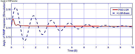
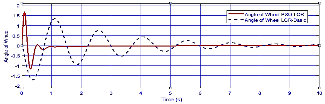
Fig. 19 and Fig. 20 illustrate a comparison of the pendulum angle responses between the LQR and PSO-LQR control strategies. The results reveal that the PSO-LQR method exhibits superior stability compared to the traditional LQR approach. Throughout the control process, the PSO-LQR maintains a consistent response with minimal fluctuations, underscoring its effectiveness. Importantly, the PSO-LQR limits the initial angle deviation to a maximum of 0.15 rad, while the LQR approach permits a more significant initial deviation of up to 0.5 rad. This limitation highlights the PSO-LQR’s capability to deliver enhanced control over the pendulum system, demonstrating its potential as a more reliable solution for stabilizing dynamic systems.

19. Angle of Pendulum response (Simualation) 

20.  Angle of Pendulum response (Experiment)

From Fig. 22 and Fig. 23 onward, the comparative analysis highlights the superior performance of the PSO-LQR method over the traditional LQR in controlling the RWIP. The PSO-LQR demonstrates significantly faster response times, stabilizing the system within 1-2 seconds, while the LQR approach tends to take up to 10 seconds to achieve similar stabilization.

Additionally, the control performance illustrated in these figures shows that the PSO-LQR maintains a more stable pendulum angle with reduced fluctuations during the control process, confirming its efficiency in ensuring system stability. The results indicate that while the LQR can effectively reduce settling time, the PSO-LQR outperforms it in overall response speed and stability.

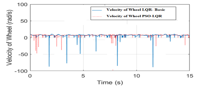
Moreover, the PSO-LQR method effectively minimizes velocity overloads in the reaction wheel, showcasing its robustness compared to LQR. This optimization of the control parameters not only enhances the performance quality but also demonstrates the resilience of the PSO-LQR system under various operational conditions.

21. Angle of Wheel response (Simulation)

22.  Angular Velocity of Wheel response (Simulation)

Fig. 23 illustrates that the velocity of the reaction wheel controlled by the traditional LQR method exhibits significant fluctuations, with peaks reaching nearly 100 rad/s during certain phases. In contrast, the PSO-LQR method produces a more stable set of parameters, resulting in quicker response times for the system. This stability underscores the effectiveness of the PSO-LQR approach in managing the dynamics of the RWIP, highlighting its superior performance compared to conventional LQR techniques.

23. Angular Velocity of Wheel Response (Experiment)

6. CONCLUSIONS

The control of the RWIP system using the LQR controller, while effective, can be further enhanced through optimization techniques like the PSO. The conventional LQR method involves manual tuning of the weighting matrices Q and R, which can be time-consuming and lacks the precision needed to achieve optimal performance across all system states. In contrast, PSO automates the process of finding optimal values for these matrices by leveraging swarm intelligence to search for the best solutions iteratively, leading to faster convergence and better overall system performance.

Compared to manual tuning or even Genetic Algorithms, PSO has distinct advantages. The PSO algorithm, inspired by the social behavior of birds, explores the search space more efficiently and focuses the swarm's efforts on the most promising solutions. This results in faster convergence and higher accuracy, as evidenced by progressively smaller values of the objective function J in larger populations. For instance, in simulations comparing populations of 5x5, 20x20, 30x30, 50x50, and 100x100 particles, PSO consistently outperforms manual tuning and GA in terms of both speed and stability.

Furthermore, PSO’s ability to limit the initial conditions more effectively than LQR—where PSO-LQR maintains a smaller initial pendulum angle deviation—demonstrates its superior control stability. In real-world applications, such as the reaction wheel’s velocity control, PSO minimizes fluctuations and accelerates system stabilization, which traditional LQR cannot achieve to the same degree. While LQR excels at reducing settling time, PSO-LQR provides a more balanced solution, optimizing both the system’s response time and stability, especially under complex and dynamic operational conditions.

In conclusion, PSO optimizes the performance of LQR controllers beyond manual methods and other algorithms like GA, offering a more efficient, robust, and adaptive solution for controlling nonlinear and dynamic systems such as the RWIP. This makes it an ideal approach for achieving precise, real-time control in practical applications where stability and fast response are critical.

Acknowledgment:

This work was supported by Posts and Telecommunications Institute of Technology, Vietnam under grant number 04-2024-HV-KTĐT2

References

1. M.F. Hamza et al, “Inverted Pendulum as a benchmark for testing linear and nonlinear control algorithms,” Mechanical Systems and Signal Processing, vol. 116, pp. 347-369, 2019, https://doi.org/10.1016/j.ymssp.2018.06.054.
2. W. Vega et al., "Conceptual Mechatronics Design and Prototyping of Autonomous Inverted Pendulum-System applied on Two-Wheeled Mobile Robot," 2023 Third International Conference on Advances in Electrical, Computing, Communication and Sustainable Technologies (ICAECT), pp. 1-6, 2023, https://doi.org/10.1109/ICAECT57570.2023.10118071.
3. V. Tudić, D. Kralj, J.  Hoster, and T. Tropčić, “Design and Implementation of a Ball-Plate Control System and Python Script for Educational Purposes in STEM Technologies,” Sensors, vol. 22, no. 5, p. 1875, 2022, https://doi.org/10.3390/s22051875.
4. Scott C. Brown, Kevin M. Passino, “Intelligent Control for an Acrobot,” Journal of Intelligent and Robotic System, vol. 18, pp. 209-248, 1997, https://doi.org/10.1023/A:1007953809856.
5. D. J. Block, K. J. Åström, K. J., & Spong, M. W. (2007). The reaction wheel pendulum (No. 1). Morgan & Claypool Publishers. 2007. https://doi.org/10.2200/S00085ED1V01Y200702CRM001.

6. H. -W. Kim, J. -W. An, H. d. Yoo and J. -M. Lee, "Balancing control of bicycle robot using PID control," 2013 13th International Conference on Control, Automation and Systems (ICCAS 2013), Gwangju, pp. 145-147, 2013, https://doi.org/10.1109/ICCAS.2013.6703879.
7. E. V. Kumar and J. Jerome, “Robust LQR controller design for stabilizing and trajectory tracking of inverted pendulum,” Procedia Engineering, vol. 64, pp. 169-178, 2013, https://doi.org/10.1016/j.proeng.2013.09.088.
8. S. Istiqphara et al., "Enhanced Equation Discovery of 3-DoF Robotic Manipulator Dynamics Using LASSO Model Selection Criteria With Variable Segregation Algorithm," in IEEE Access, vol. 12, pp. 20574-20590, 2024, https://doi.org/10.1109/ACCESS.2024.3354374.
9. A. Sutradhar et al., "Identification of servo-driven inverted pendulum system using neural network," 2010 Annual IEEE India Conference (INDICON), pp. 1-4, 2010, https://doi.org/10.1109/INDCON.2010.5712589.
10. S. Howimanporn et al., “Design and Implementation of PSO Based LQR Control for Inverted Pendulum through PLC,” IEEE/SICE International Symposium on System Integration, pp. 13-15, 2016, https://doi.org/10.1109/SII.2016.7844075.

11. M. Benedetti, R. Azaro, D. Franceschini, A. Massa, "PSO-Based Real-Time Control of Planar Uniform Circular Arrays," IEEE Antennas and Wireless Propagation Letters, vol. 5, no. 1, pp. 545 548, 2006, https://doi.org/10.1109/LAWP.2006.887553.
12. A. Ibrahim, N. Hassan, O. Shomer, “Optimal PID control of a brushless DC motor using PSO and BF techniques,” Ain Shams Eng, vol. 5, no. 2, pp. 391–398, 2014, https://doi.org/10.1016/j.asej.2013.09.013.
13. R. Yazgan et al., “Comparison performances of PSO and GA to tuning PID controller for the DC motor,” Sakarya Univ. J. Sci., vol. 23, no. 2, pp. 162–174, 2019, https://doi.org/10.16984/saufenbilder.376464.
14. F. Loucif et al., “Whale optimizer algorithm to tune PID controller for the trajectory tracking control of robot manipulator,” J. Braz. Soc. Mech. Sci. Eng., vol. 42, no. 1, pp. 1–11, 2020, https://doi.org/10.1007/s40430-019-2074-3.
15. M. Juneja and S. K. Nagar, "Particle swarm optimization algorithm and its parameters: A review," 2016 International Conference on Control, Computing, Communication and Materials (ICCCCM), pp. 1-5, 2016, https://doi.org/10.1109/ICCCCM.2016.7918233.  
16. P. L. Nguyen, et al., “Adaptive Evaluation of LQR Control using Particle Swarm Optimization for Pendubot,” Journal of Fuzzy Systems and Control, vol. 2, no. 2, pp. 58-66, 2024, https://doi.org/10.59247/jfsc.v2i2.203.