Backstepping Control for Ball and Beam: Simulation and Experiment

Vo-Hoang-Lap Tran 1, Trung-Hieu Le 2, Dai-Phuc Hoang 3, Van-Dong-Hai Nguyen 4, Ngoc-Thinh Ho 5, Tien-Phat Do 6, Tuan-Cuong Le 7, Thi-Xuan-Hy Tran 8, The-Duy Luong 9, Thanh-Son Vo 10, Phuoc-Khanh Nguyen 11, Minh-Tam Nguyen 12,*

1, 2, 3, 4, 5, 6, 7, 8, 9, 10, 11, 12 Ho Chi Minh City University of Technology and Education (HCMUTE), Ho Chi Minh City, Vietnam

Email: 1 20151389@student.hcmute.edu.vn, 2 @20151368student.hcmute.edu.vn, 3 20145301@student.hcmute.edu.vn,

4 hainvd@hcmute.edu.vn, 5 21161015@student.hcmute.edu.vn, 6 21161468@student.hcmute.edu.vn,

7 21161432@student.hcmute.edu.vn, 8 21161323@student.hcmute.edu.vn, 9 19145212@student.hcmute.edu.vn,

10 19145300@student.hcmute.edu.vn, 11 19145075@student.hcmute.edu.vn, 12 tamnm@hcmute.edu.vn 

*Corresponding Author

Abstract—This paper presents the modeling and control of the Ball and Beam system, a commonly used Single Input – Multiple Output (SIMO) system in control research experiments. In the study, the Backstepping method is applied to model and control the system. The linear differential equations describing the system's dynamics are derived based on fundamental mechanical principles, using the Euler-Lagrange method to develop an accurate mathematical model. Subsequently, the backstepping method is employed to design a controller that ensures the global stability of the system. Lyapunov theory is applied to prove the system's stability, with an appropriate Lyapunov function selected to guarantee the global stability of the controller. In addition to simulations, the study also conducts experiments to test the system's stability under Backstepping control. The results show that this controller is not only effective in maintaining balance and controlling the position of the ball on the beam but also addresses the limitations of traditional linear control methods. Both simulation and experimental results demonstrate the high performance and stability of the system, confirming the stability according to Lyapunov theory.

Keywords—Backstepping Control, Ball and Beam, Linear Control, SIMO Systems

1. Introduction

In the field of control and automation, many real-world systems exhibit a nonlinear nature, presenting significant challenges for analysis and control. This nonlinearity makes such systems unpredictable, requiring advanced analytical techniques and sophisticated control methods to maintain stability and efficiency in operation [1]-[2]. Nonlinear systems are often studied in academic settings as a learning and experimental tool, providing students and researchers with valuable opportunities to develop the skills necessary to address practical control issues.

In educational contexts, the ball-and-beam system is a quintessential example of a nonlinear and unstable system, commonly used to illustrate advanced control concepts [3]. This system consists of a beam that can rotate around an axis, on which a ball moves. The operator must adjust the beam’s angle to keep the ball at a desired position, a challenging task due to the nonlinear relationship between the ball’s position and the beam’s angle. Classical control methods like PID [4] have been applied to this system, alongside optimal control methods such as the Linear Quadratic Regulator (LQR) [5]. However, the nonlinearity and high precision required demand more advanced control approaches.

Numerous studies have proposed and applied advanced control methods to the ball-and-beam system to enhance stability and control efficacy. Specifically, state-space control has been explored in [6] with centrifugal force equations to build adaptive control rules, while adaptive fuzzy control has been used in [7] to manage balancing with dynamic surface optimization strategies. Nonlinear backstepping control [8] and sliding mode control (SMC) were combined in [9] to create a robust strategy, with SMC applied to both static and dynamic configurations. Additionally, in [10], Jacobian-based SMC was employed to linearize the system, and an integral SMC approach has been implemented for this system in [11]. A study has compared various SMC strategies, such as first-order, second-order (super-twisting), fast control, and integral control, to enhance system tracking performance [12].

Other studies have utilized PD controllers for precise compensation, combined with neural network controllers to approximate nonlinear elements [13]. In [14], the extended kalman filter (EKF) was used to improve stability by accurately estimating neural controller weights. Fuzzy control with genetic algorithm optimization for cascade controller design [15], and cascade PD fuzzy control with particle swarm optimization in [16]. Methods like input-output linearization via approximation [17] and two-degree-of-freedom (DOF) model control [18] were also researched to increase efficiency in ball-and-beam control applications.

In this research, we focus on applying the linear backstepping method to stabilize the ball-and-beam system. The backstepping approach is regarded as an effective technique for designing controllers with clear structures and ensuring local stability for the system. However, since this method relies on linearizing the system around an equilibrium point, it is effective only within a limited range around that point. As the ball moves away from the equilibrium position, or when disturbances occur, this method can no longer guarantee stability, which highlights a limitation that current research needs to address.

While the linear backstepping method provides efficacy within a certain range, its limitations reveal a significant gap in the literature regarding the broader application of nonlinear control methods. Modern nonlinear control techniques, such as adaptive control and sliding mode control, are gaining attention for their ability to handle highly nonlinear systems. However, comprehensive studies evaluating the performance of these methods on the ball-and-beam system are still lacking, especially in academic and educational settings where nonlinear control methods can enhance learners’ understanding.

Therefore, this study not only aims to verify the effectiveness of the linear backstepping method but also to explore its limitations in controlling the nonlinear ball-and-beam system. This research contributes to the literature on control methods for unstable systems, further clarifying the operational scope limitations of the backstepping method as discussed in [19]. Additionally, the study will suggest new directions for nonlinear control methods, such as adaptive control or sliding mode control, with the aim of enhancing the comprehensiveness of control systems in nonlinear environments.

2. Mathematical Model

The ball and beam system is a SIMO configuration, in which a ball rolls freely along the length of the beam. The system consists of two critical components: a motor that controls the rotational angle of a disk, thereby altering the tilt of the beam, and the ball-beam assembly itself. This system operates with two degrees of freedom, where the ball moves translationally along the horizontal axis of the beam, while the beam oscillates vertically with one end fixed. The beam's angle shifts in response to the torque exerted by the motor can be seen in Fig. 1.

1. Modeling the system [20]

To derive the equations describing the motion of the ball and beam system, based on the reference [21], the Lagrange method based on energy balance is used [22]. At the same time, combined with the method for finding the nonlinear equations of the ball and beam system mentioned in [23] and [24], the authors' group derived the equations describing the system's motion.

First, we need to determine the kinetic energy of the system, which consists of two components: the kinetic energy of the beam and the kinetic energy of the ball.

• The kinetic energy of the ball is comprised of two parts:

Translational kinetic energy:

Rotational kinetic energy:

• The kinetic energy of the beam:

The beam only possesses rotational kinetic energy.

           The total kinetic energy of the system:

The potential energy of the system:

The potential energy of the ball:

The potential energy of the beam:

The total potential energy of the system:

According to the Lagrange formula:

From (8)

Upon expanding the Lagrange equation, it will take the following form

  From (10), it follows that:

We proceed by differentiating equation (9) as in equation (11) and equation (12).

Finally, after simplification, the mathematical model of the ball and beam system is expressed as follows:

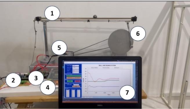
The parameters obtained from the physical model, depicted in Fig. 9, are listed in Table 1.

1. Parameters of the System

The angles  and   are related to each other as described in document [4]. From angle , we can infer  using the formula below:

To control the torque of the motor, we need to manage its voltage. According to document [25], there is a relationship between torque and voltage. Based on the mathematical equations describing torque and the input voltage of the system from document  [25], we proceed to identify the motor parameters to apply the equations to the physical model.

        With the relationship between torque and voltage, we substitute into equation (15), (16), and (17) to obtain the following equation:

To linearize the system, it is necessary to construct a state-space model, in which =.

Define the state variables as follows:

The system in the state-space equations is represented as follows:

We set the values as follows:

We can compute the matrices A and B using the model parameters provided in Table 1. Nonlinear system is considered to operate only around an equilibrium point:

3. Controller

1. Linear Backstepping Control

The backstepping algorithm referenced from document [26] is applied to system , where we formulate a control law to stabilize the system. According to document [26], the virtual control functions are designed such that the subsystems become stable. Based on Lyapunov’s theory [27], the system's control law is developed through four steps, which are outlined below.

For the ball and beam system, we convert it into a state-space model using state variables.

Step 1: The first step in designing the linear backstepping controller is to define an error variable, which is specified as follows:

Wherein,  represents a constant specific to the system. We compute the derivative of as follows:

Step 2: To guide the control law  toward zero, we consider  as a virtual control variable. A positive definite Lyapunov function is selected as follows:

According to Lyapunov's criterion, an appropriate function must be chosen to satisfy the condition . Thus, the derivative of  is given as follows:

From Appendix (A1), we define the functionin such a way as to ensure system stability as follows:

Where  is a positive constant.

Step  3: The next error variable, is defined as follows:

The derivative of is calculated as follows:

Substituting equation (24) into equation (31), we obtain:

Substituting equation (26) into equation (32), we obtain:

We set:

Rewrite equation (33) as follows:

Step  4: To ensure that the function  is truly stable, we consider . The goal of this step is to select a function such that , and the function must include , defined as follows:

From equation (30) to equation  (26), we have:

The derivative of  yields the following equation:

Substituting (37) into (38), the equation becomes:

To ensure is negative in accordance with Lyapunov stability theory, we define  as follows:

Where is a positive constant designed for the system. Substituting (40) into (39) yields the following form:

We substitute equations (25), (30), and (35) into (40). From this equation, we derive the control law as follows

Where  is a design constant of the system

2. Evaluation of Stability of the Backstepping Controller

We evaluate the performance and stability of the backstepping controller based on Lyapunov theory, with the Lyapunov function  considered as follows:

When taking the derivative of , we obtain the following result:

By substituting functions (26), (40), and (37) into (44), we obtain:

Based on the outcomes obtained from (45), it is certain that the system can achieve stability. By satisfying the Lyapunov function conditions from (43) and (45), the system can stabilize as it asymptotically converges to zero as time approaches infinity.

When the error variable tends to zero, indicating that the system has reached a stable state, it can also be observed that both variables  and  have attained the desired positions within the system.

4. Results and Discussion

In this study, the backstepping controller is employed to stabilize and control the ball and beam system, a nonlinear system characterized by the intricate interactions between the ball and the beam. Simulations and experiments are conducted to demonstrate the feasibility, accuracy, and performance of the controller, allowing for a comparison with alternative control methods and an assessment of the advantages and disadvantages under practical operating conditions.

3. Simulation Results

In this simulation section, the authors will model the system using the Matlab – Simulink tool, which allows us to simulate the system based on the mathematical equations derived using the Lagrangian method. We will implement the simulation of the system with the Backstepping controller identified in the preceding section. The parameters for the simulation are based on Table 1, which we derived from the physical model to ensure that the simulation results are visually meaningful.

In the simulation, we initialize the starting position for Ball and Beam based on the physical model as follows:

The simulation duration for the system is 100 seconds, and the sampling time is 0.01 seconds.

Functional blocks are constructed in Matlab Simulink, as shown in Fig. 2 and Fig. 3, with the following purposes:

Block 1: This block serves to provide reference signals for the system (e.g., sine waves, square pulses, etc.).

Block 2: This is backstepping controller, which is responsible for collecting input data and generating control signals for actuator, enabling system to achieve desired position.

Block 3: This block represents the actuator of the system, which has been modeled. It describes the motion of the system in response to the control signals.

Block 4: Final block is scope block, which collects data from Matlab Simulink and allows us to visualize the data.

2. Block 1 and block 2 in Matlab/Simulink

3. Block 3 and block 4 in Matlab/Simulink

Table 2 are the parameters of the controller:

2. The control parameters

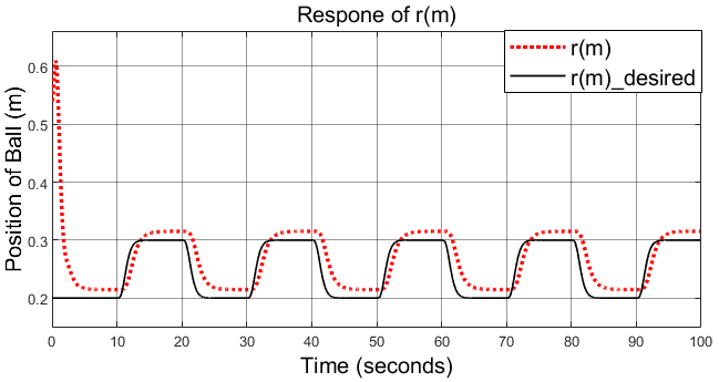
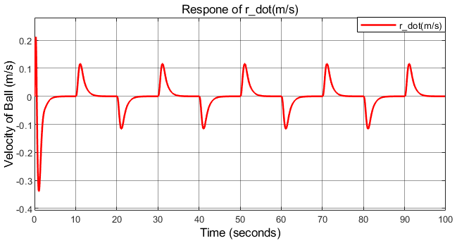
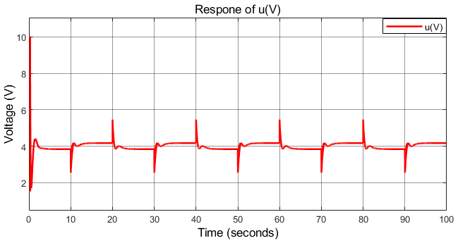
The simulation results, including r (m),  (rad), and voltage (V), are presented from Fig. 4 to Fig. 8 The initial values of the system are as follows:

4. Position of ball (m)

5. Velocity of ball (m/s)

The authors simulated the Ball and Beam system, with the results displayed from Fig. 4 to Fig. 8, respectively showing the ball position, ball speed, beam angle, beam angular velocity, and finally the control signal, which in this case is the motor voltage. We had the ball follow a square wave trajectory with an amplitude ranging from 0.2m to 0.3m to evaluate the system’s stability.

6. Angle of beam (rad)

7. Angle Velocity of beam (rad/s)

8. Control signal

From this, it can be seen that the system was stable, with no overshoot, and the ball’s settling time was 5.6 seconds. However, although the ball followed the square wave trajectory, there was still a certain error of about 0.03m. This indicates that during the system's linearization process, some changes occurred, leading to slight discrepancies. In summary, with the obtained control signal (Fig. 8), the authors successfully simulated the backstepping controller.

4. Experimental Results

Below is the hardware model of the Ball and Beam system used for experimentation. The components of the actual system are divided into six parts, as shown in Fig. 9, which include:

1. Beam
2. DC Motor
3. STM 32F407VG Microcontroller
4. HI216 H-Bridge
5. 220 VAC Power Supply
6. Lever Arm
7. Graphical user interface

9. Physical model in HCMUTE

After conducting the simulation, we proceeded to test the controller on the physical model to verify its stability. The experimental results we have just published, from Fig. 10 to Fig. 14, show the actual ball position, actual ball speed, actual beam angle, actual beam angular velocity, and finally the actual control signal, respectively. Similar to the simulation, we had the ball follow a square wave trajectory to validate the controller.

Regarding the system's performance, as shown in Fig.10, it is clear that the ball closely followed the square wave trajectory, achieving a settling time of 5.8 seconds with an acceptable error margin. However, some noise was present, and we also observed that the signals obtained from the real experiments showed a relatively high degree of similarity.

 Therefore, it can be concluded that the process of identifying the system from the physical model to the mathematical equations demonstrates significant reliability. The experimental results indicate that our team successfully implemented the linear backstepping algorithm for the ball and beam system in both simulation and real-world applications.

10. The position of the ball during experimentation

11. The velocity of the ball during experimentation

12. The angle of the bem during experimentation

13. The velocity angle of the bem during experimentation

14. Control signal

1. Discussion

During the design process of the controller, we identified several noteworthy points. First, in the modeling of the system, we neglected external forces acting on it, specifically frictional forces, in order to simplify the calculations. However, this omission also affects the quality of our controller. Nevertheless, this can potentially be compensated for by employing a robust controller.

Next is the backstepping controller, where the virtual variables in the controller are based on several references mentioned during the designing process. Since these virtual variables are defined to satisfy the Lyapunov theorem, the variabledepends on , making the system more challenging to stabilize. However, according to the principle that when  approaches zero,  will also approach zero. Therefore, whenstabilizes, the entire system stabilizes as well.

Contributing factor is the unique structure of the ball and beam system, where and, or and , are interdependent. When the angle  reaches its equilibrium value, the beam remains still, causing the ball to also remain stationary, thereby making the system easier to stabilize. Finally, since the controller we designed is a nonlinear controller, model errors still exist. To address this, a nonlinear controller  specifically designed for the ball and beam system could be implemented [28].

5. Conclusion

This article presents the design of a linear controller using the backstepping method to control the position of the ball in a ball-and-beam dynamic system. The design procedures are described in detail, and both simulation and experimental results show that, although the backstepping controller performs well, there is still a certain degree of error due to its linear nature.

The linear backstepping controller has several advantages, such as ensuring system stability and accuracy through Lyapunov theory, effectively handling nonlinear systems, and being adaptable in dynamic environments. However, it also has some drawbacks, such as the need for an accurate model, difficulty in real-world implementation, and the requirement for in-depth knowledge during the design process. Furthermore, its performance may degrade when faced with strong disturbances or complex systems, particularly when the linear model does not fully capture the nonlinear behavior of the actual system. This was clearly demonstrated during testing.

To address these issues, the controller parameters can be fine-tuned using optimization algorithms such as Particle Swarm Optimization (PSO) or Genetic Algorithm (GA), and noise reduction filters can be added to the system to improve control quality.

Additionally, designing a nonlinear backstepping controller is a promising approach to significantly reduce system errors and enhance control performance. To further improve the system, intelligent controllers such as fuzzy controllers, neural networks, or predictive models could be incorporated to anticipate system behavior, thereby increasing adaptability and optimizing the control process. These methods not only make the system more flexible but also enhance control performance, especially when dealing with unexpected changes or complex operating conditions.

ACKNOWLEDGEMENT

This paper belongs to project of students of Ho Chi Minh City University of Technology and Education (HCMUTE) for year 2025. It is funded by HCMUTE. We, authors, want to give thanks to that support.

Appendix a

The derivative of (27):

We will choose a function that satisfies (45)

We select a function that ensures the stability of (45) according to Lyapunov's theory:

References

1. A. Y. Krasinskiy et al., "Modeling of the ball and beam system dynamics as a nonlinear mechatronic system with geometric constraint," estnik Udmurtskogo Universiteta. Matematika. Mekhanika. Komp'yuternye Nauki, vol. 27, no. 3, pp. 414-430, 2017,  https://doi.org/10.20537/vm170310.
2. A. A. Ezzabi et al., "A nonlinear backstepping control design for ball and beam system," in 2013 IEEE 56th International Midwest Symposium on Circuits and Systems (MWSCAS), pp. 1318-1321, 2013, https://doi.org/10.1109/MWSCAS.2013.6674898.
3. F. Lamnabhi-Lagarrigue et al., "Systems & control for the future of humanity, research agenda: Current and future roles, impact and grand challenges," Annual Reviews in Control, vol. 43, pp. 1-64, 2017,  https://doi.org/10.1016/j.arcontrol.2017.04.001.
4. V.-C. Pham et al., "GA-PID Control for Ball and Beam: Simulation and Experiment,” Robotica & Management, vol. 27, no. 2, 2022,  https://doi.org/10.24193/rm.2022.2.5.
5. A. Umar et al., "Performance Comparison of the Ball and Beam System using Linear Quadratic Regulator Controller," in PID Control for Linear and Nonlinear Industrial Processes, 2023,   https://doi.org/10.5772/intechopen.110513.

6. Y. Sahu et al., "Optimal PD-PD and State Feedback Control of Underactuated Ball and Beam System with Uncertainty and Disturbances," in International Conference on Mathematical Modeling in Physical Sciences, pp. 87-104, 2023, https://doi.org/10.1007/978-3-031-52965-8_7.
7. R. Chotikunnan et al., "Ball and beam control: evaluating type-1 and interval type-2 fuzzy techniques with root locus optimization," International Journal of Robotics and Control Systems, vol. 3, no. 2, pp. 286-303, 2023,  http://dx.doi.org/10.31763/ijrcs.v3i2.997.
8. M. F. Rahmat et al., "Application of intelligent controller in a ball and beam control system," International journal on smart sensing and intelligent systems, vol. 3, no. 1, pp. 45-60, 2010,  https://doi.org/10.21307/ijssis-2017-378.
9. N. B. Almutairi and M. Zribi, "On the sliding mode control of a ball on a beam system," Nonlinear dynamics, vol. 59, pp. 221-238, 2010,  https://doi.org/10.1007/s11071-009-9534-8.
10. X. Li and W. Yu, "Synchronization of ball and beam systems with neural compensation," International Journal of Control, Automation and Systems, vol. 8, pp. 491-496, 2010,  https://doi.org/10.1007/s12555-010-0301-x.

11. S. ud Din et al., "Robust control of underactuated systems: Higher order integral sliding mode approach," Mathematical problems in engineering, vol. 2016, no. 1, p. 5641478, 2016,  https://doi.org/10.1155/2016/5641478.
12. S. U. Din et al., "A comparative experimental study of robust sliding mode control strategies for underactuated systems," IEEE Access, vol. 5, pp. 10068-10080, 2017,  https://doi.org/10.1109/ACCESS.2017.2712261.
13. R. M. Hirschorn, "Incremental sliding mode control of the ball and beam," IEEE Transactions on Automatic Control, vol. 47, no. 10, pp. 1696-1700, 2002,  https://doi.org/10.1109/TAC.2002.803538.
14. P. H. Eaton et al., "Neurocontroller alternatives for" fuzzy" ball-and-beam systems with nonuniform nonlinear friction," IEEE transactions on Neural Networks, vol. 11, no. 2, pp. 423-435, 2000,  https://doi.org/10.1109/72.839012.
15. S.-K. Oh et al., "The design of a fuzzy cascade controller for ball and beam system: A study in optimization with the use of parallel genetic algorithms," Engineering Applications of Artificial Intelligence, vol. 22, no. 2, pp. 261-271, 2009,  https://doi.org/10.1016/j.engappai.2008.07.003.

16. S.-K. Oh et al., "Optimized fuzzy PD cascade controller: A comparative analysis and design," Simulation Modelling Practice and Theory, vol. 19, no. 1, pp. 181-195, 2011,  https://doi.org/10.1016/j.simpat.2010.06.004.
17. J. Hauser et al., "Nonlinear control via approximate input-output linearization: The ball and beam example," IEEE transactions on automatic control, vol. 37, no. 3, pp. 392-398, 1992,  https://doi.org/10.1109/9.119645.
18. W. Yu, "Nonlinear PD regulation for ball and beam system," International Journal of Electrical Engineering Education, vol. 46, no. 1, pp. 59-73, 2009,  https://doi.org/10.7227/IJEEE.46.1.5.
19. V.-T. Do et al., "Robust integral backstepping hierarchical sliding mode controller for a ballbot system," Mechanical Systems and Signal Processing, vol. 144, p. 106866, 2020,  https://doi.org/10.1016/j.ymssp.2020.106866.
20. R. S. Shekhawat and N. Singh, "Application of Reinforcement Learning in Control Systems for Designing Controllers," in Machine Intelligence and Smart Systems, 2022, ch. Chapter 9, pp. 117-128  https://doi.org/10.1007/978-981-16-9650-3_9.

21. P. M. Maalini et al., "Modelling and control of ball and beam system using PID controller," in 2016 International Conference on Advanced Communication Control and Computing Technologies (ICACCCT), pp. 322-326, 2016,  https://doi.org/10.1109/ICACCCT.2016.7831655.
22. M. Keshmiri et al., "Modeling and control of ball and beam system using model based and non-model based control approaches," International Journal on smart sensing and intelligent systems, vol. 5, no. 1, pp. 14-35, 2012,  https://sciendo.com/pdf/10.21307/ijssis-2017-468.
23. J. Schoukens and L. Ljung, "Nonlinear system identification: A user-oriented road map," IEEE Control Systems Magazine, vol. 39, no. 6, pp. 28-99, 2019,  https://doi.org/10.1109/MCS.2019.2938121.
24. S. L. Brunton, J. L. Proctor, and J. N. Kutz, "Discovering governing equations from data by sparse identification of nonlinear dynamical systems," Proceedings of the national academy of sciences, vol. 113, no. 15, pp. 3932-3937, 2016,  https://doi.org/10.1073/pnas.1517384113.
25. B. Hamza et al., "A New method for the parametric identification of DC machines using MATLAB identification toolbox and experimental measurements," in E3S Web of Conferences, vol. 336, p. 00007, 2022,  https://doi.org/10.1051/e3sconf/202233600007.

26. M. T. Vo et al., "Back-stepping control for rotary inverted pendulum," Journal of Technical Education Science, vol. 15, no. 4, pp. 93-101, 2020,  https://jte.edu.vn/index.php/jte/article/view/110.
27. C. Aguilar-Ibañez, "On the stabilization of the ball and beam system using a direct Lyapunov method," in 2009 6th International Conference on Electrical Engineering, Computing Science and Automatic Control (CCE), pp. 1-6, 2009,  https://doi.org/10.1109/ICEEE.2009.5393462.
28. A. Singh and H. K. Khalil, "Regulation of nonlinear systems using conditional integrators," International Journal of Robust and Nonlinear Control: IFAC‐Affiliated Journal, vol. 15, no. 8, pp. 339-362, 2005,  https://doi.org/10.1002/rnc.996.