An LQR-Based ANFIS Control for Double-Linked Inverted Pendulum on Cart

Truong-Phuong-Nam Pham 1, Trong-Bang Tran 2, Van-Dong-Hai Nguyen 3, Tai-Tue Nguyen 4, Gia-Thinh Nguyen 5,

Duy-Phat Nguyen 6, Dong-Khang Nguyen 7, Van-An Ha 8, The-Nam-Chau Trinh 9, Trung-Thang Nguyen 10,*

1,3,4,5,6,7,8,9,10 Ho Chi Minh City University of Technology and Education (HCMUTE), Ho Chi Minh City (HCMC), Vietnam

2 Department of Mechanical Engineering, Konkuk University, Seoul 05029, Republic of Korea

10 Cao Thang Technical College, Vietnam

Email: 1 22151119@student.hcmute.edu.vn, 2 bang11111@konkuk.ac.kr, 3 hainvd@hcmute.edu.vn,

4 21151490@student.hcmute.edu.vn, 5 20151004@student.hcmute.edu.vn, 6 21144346@student.hcmute.edu.vn,

7 21145161@student.hcmute.edu.vn, 8 21145624@student.hcmute.edu.vn, 9 21145082@student.hcmute.edu.vn,

10 nguyentrungthang@caothang.edu.vn 

*Corresponding Author

Abstract—This paper presents a double-linked inverted pendulum on a cart system, which is highly nonlinear and inherently unstable. In the simulation, the state variable outputs are processed through three ENCODER blocks with a resolution of 1000 pulses, as we aim to develop a mathematical model that closely approximates real-world experiments. The objective of this study is to use an ANFIS controller to learn from data that closely resembles the actual system behavior under an LQR controller and apply it in a simulation environment to evaluate the stability and response of the system under both ANFIS and LQR controllers. The results show that the ANFIS controller provides better responses than the LQR controller.

Keywords—ANFIS Control; LQR Control; Intelligent Control; SIMO System; Double-Linked Inverted Pendulum

1. Introduction

The inverted pendulum (IP), characterized by its under-actuated, non-linear, and unstable nature, has been extensively studied by numerous researchers. These studies aim to analyze the behavior and assess the performance of various novel and traditional control algorithms [1].

Many approaches have been effectively implemented to control the double-linked inverted pendulum. For example, PID controllers have been used to stabilize the system [2]-[4]. Other methods include the application of fuzzy controllers [5], as well as optimal control techniques utilizing LQR controller for controlling the double-linked inverted pendulum [6]-[9].

This research focuses on developing a standardized and systematized process for deriving dynamic equations by integrating advanced mathematics, classical physics, and robot motion analysis. Specifically, using data from John Gray's forward kinematics, we apply mathematical techniques to generate equations related to positions, angular velocities, and linear velocities. Based on these, the potential energy and kinetic energy equations are constructed efficiently. Finally, by employing the Euler-Lagrange equation, the dynamic equations are derived in a straightforward manner [10].

ANFIS (Adaptive Neuro-Fuzzy Inference System) is a hybrid intelligent system that combines fuzzy logic and artificial neural networks (ANNs) to enhance learning and inference capabilities. It was introduced to take advantage of both techniques, providing a powerful tool for modeling complex nonlinear systeam. By using a hybrid learning procedure, the proposed ANFIS can construct an input-output mapping based on both human knowledge (in the form of fuzzy if-then rules) and stipulated input-output data pairs [11]. ANFIS has been effectively applied in learning various control methods including PID, LQR, and nonlinear control [12]-[16]. It has been implemented on systems that are considered iconic in control algorithm research within the field of automation in particular and electrical-electronics engineering in general.

In this paper, the authors first develop a mathematical model of the system and then perform simulations using both a fuzzy controller and an LQR controller. These algorithms are later tested through simulations.

2. Mathematical Equations and Simulation

1. Mathematical Equations

To begin with, we analyze system to build up the motion of the whole system. Basically, the overall analyzation is shown in the Fig. 1.

1. Basic structure of the system

Experience in setting and assigning system parameters has been inherited from research documents on pendubot. Our previous experimental studies on this model, as presented in various publications, demonstrate that analyzing the system's dynamic equations using the Euler–Lagrange method provides high accuracy and closely approximates the real model. The parameters in Table 1 are measured and identified from our actual model.

1. Parameters of system

However, this method presents a significant challenge as it has not been systematically structured to establish relationships between state variables when calculating kinetic and potential energy. These relationships are often determined through geometric methods, which can be difficult to apply to higher-order systems. Our proposed solution is to utilize the forward kinematic computation method from robotics, based on the algebraic approach introduced by John J. Craig [10].

2. Forward Kinematic

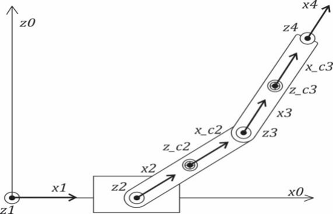
The coordinate system is defined as shown in Fig. 2, where we introduce additional coordinate frames c2 and c3 to determine the center of mass of the pendulums.

2. Axis system of joints in the system

From the axis system in Fig. 2, the DH table is filled in Table 2. In there, the condition parameters are , and ; the rests are constant parameters.

2. DH table of system

This table is constructed following the Denavit–Hartenberg (DH) convention as introduced in [10]. In Table 2, the DH parameters are chosen based on the configuration of the double-linked pendulum system.

Next stage, T identity matrix is being derived in the equation (1) base on the formula in [10].

With parameters from DH table, T matrixes are written as:

Coordinates of the centers of gravity of the joints with reference to the previous joint.

To determine the coordinates of each joint, we multiply in turn as follows:

3. Dynamic Equations

1. Linear Velocity and Angular Velocity

To find the system kinetic energy, we need the linear velocity and angular velocity at the center of gravity of each pendulum. Regarding the linear velocity, we need to determine the center of gravity of each pendulum and the cart through the equations (12), (13) and (14).

After that, linear velocity is derivative of coordinates with respect to time.

In terms of the angular velocity, base on the analyzation from document [10] the vector x of each pendulum can be determined through the matrix below.

Angular velocity is determined by the derivative of vector x matrix with respect to time.

2. Euler – Lagrange Equations

This equation consists of two components  (kinetic energy) and  (potential energy). Theoretically, it is presented in the format.

Regard to the kinetic energy, it is total kinetic energy of cart and 2 poles.

Similarly with potential energy, the total potential energy is shown below.

From Euler-Lagrange equation (24):

The general form of the state equation, when systematized, is as follows:

The acceleration equation is rewritten from the state equation as follows:

Where:

With:

Thence, we obtain:

Linearizing the system, we obtain:

From the model, we can calculate matrix A, B

The system is discretized using a sampling period of 5 milliseconds.

3. Controller

1. LQR

The inverted pendulum on a cart system is described by the linear state-space equation as follows:

With:

:

:

In which:

 Applied force on cart

 Torque acting on the first pendulum

 Torque acting on the second pendulum

Objective is to determine the input vector ‘u’, so as to

minimize the performance index:

In which:

Q is a positive-semi definite and R is a positive definite matrix. Here the elements of the matrix u are determined, so as to minimize the performance index. Then  is optimal for any initial state x(0). Where P is the solution of Riccati equation, K is the linear optimal feedback matrix. Now we only need to solve the Riccati equation [12].

Where Q and R are determined by the genetic algorithm Q=diag([0.422465 53.3543 2.077422 1.3516 4.709233 43.886800]), R= 0.842308.

Therefore,

The gain matrix 𝐾 is computed using the discrete-time LQR method via MATLAB’s function:

The computed state feedback gain matrix K is K1= 0.6162; K2= 7.4389; K3= -51.6704; K4= -23.9153; K5= -211.4428; K6= -38.9656.

Fig. 3 illustrates the block diagram of the LQR controller used in this study. In the diagram, x is the state vector, u is the control input, and y is the output vector. The feedback gain matrix K is designed to minimize a quadratic performance index as defined in Equation (49). This structure follows the standard LQR formulation, as described in [12].

3. LQR controller structure

1. LQR Based ANFIS Controller

First, we collect the input and output data of the system

when using the LQR controller. We gather 2001 samples of input data and state variables with a sampling time of 0.05s over a duration of 10 seconds. The initial conditions are set to . After collecting the data, we load it into anfisedit toolbox available in MATLAB, as shown in Fig. 4.

The FIS file using three Trimf membership functions for each input and constant output is generated in anfisedit. Finally, we train the FIS file with hybrid learning, setting the error tolerance to zero and the number of epochs to 29. The training error converges and no longer changes at the threshold of 0.0038119 as shown as Fig. 5.

4. Loaded training data plot in anfisedit

5. Training error plot in anfisedit

The final ANFIS network structure is shown in Fig. 6. The control rule surface view of ANFIS controller is shown in Fig. 7.

6. ANFIS network structure

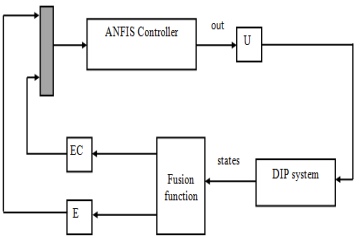
The ANFIS control structure is designed and shown in Fig. 8. This figure illustrates the ANFIS control structure, which combines fuzzy logic and neural networks to control the double-linked inverted pendulum system. This structure takes input data, processes it through fuzzy rules, and generates a control signal to stabilize the system.

7. Control rule surface view of the ANFIS controller

8. ANFIS control structure [12]

1. Simulation Program

System overview:

An overview of the blocks representing the system in the simulation environment is presented in Fig. 9.

9. Simulation of the DIPC system

Cart’s Encoder:

The encoder block simulates a real encoder with a resolution of 1000 pulses. The cart’s position output is fed into the encoder block and converted into meters for rounding calculations to minimize errors. It is then converted back into pulses and output, shown in Fig. 10.

Encoder of the first and second pendulum:

The encoder block simulates a real encoder with a resolution of 1000 pulses. The output of the angular deviation of the two pendulums is fed into the encoder block and converted into meters for rounding calculations to minimize errors. It is then converted back into pulses and output, shown in Fig. 11.

10. Simulation of the cart’s encoder

11. Simulation of the enclosure for the two pendulums

The LQR control system structure is shown in Fig. 12.

12. Simulation of the system with an LQR controller

The ANFIS control system structure is shown in Fig. 13.

13. Simulation of the system with an ANFIS controller

4. Results and Discussion

The response results of the double-linked inverted pendulum on cart system under the ANFIS and LQR controllers are shown in the four figures, corresponding to the cart position, the deviation angle of the first pendulum, the deviation angle of the second pendulum, and the applied force on the cart.

As mentioned above, we aim for a simulation environment that closely resembles real-world conditions. Therefore, the system's output has been connected to simulation blocks representing an ENCODER with a resolution of 1000 pulses. As a result, the system's response will exhibit oscillations around the equilibrium position.

Fig. 14 illustrates the cart's position response. The red line, representing the cart position using the LQR controller, oscillates within the range of -0.08 meters to 0.16 meters. This oscillation amplitude is not excessively large and remains within an acceptable range. In contrast, the black line, which represents the response of the ANFIS controller, shows a smaller oscillation amplitude compared to LQR and appears more stable. This indicates that ANFIS has learned from LQR's operation and even provides a better response than LQR.

Fig. 15 illustrates the deviation angle of the first pendulum. The red line represents the angular displacement when utilizing the LQR controller, maintaining stability within an oscillation range of -0.06 radians to 0.06 radians (equivalent to ±3.43 degrees). This oscillation amplitude is well within acceptable limits for practical implementation. The black line depicts the response of the ANFIS controller, exhibiting a comparable amplitude to the LQR-based system. This indicates that ANFIS has effectively learned and replicated the dynamic behavior of the LQR controller.

14. The response to the cart’s position

15. The response of the first pendulum

Fig. 16 illustrates the angular deviation of the second pendulum. The red line represents angular displacement when using the LQR controller, maintaining stability within an oscillation range of -0.03 radians to 0.03 radians (equivalent to ±1.72 degrees). This oscillation amplitude is relatively small compared to the first pendulum, indicating improved damping characteristics. The black line represents the response of the ANFIS controller, which exhibits a similar oscillation range to LQR but with slightly higher oscillatory energy. This suggests that ANFIS has effectively learned the control strategy of LQR, though minor residual oscillations remain.

16. The response of the second pendulum

Fig. 17 illustrates the control force applied to the cart. The force generated by the LQR controller oscillates within a range of ±10N, which leads to significant cart oscillations due to strong actuation. However, the ANFIS controller has effectively learned the control behavior of LQR and has even outperformed it by reducing the applied force, resulting in less oscillation of the cart. This is a positive outcome for the ANFIS controller, as it contributes to reducing control energy consumption while maintaining system stability.

17. The response of the applied force on the cart

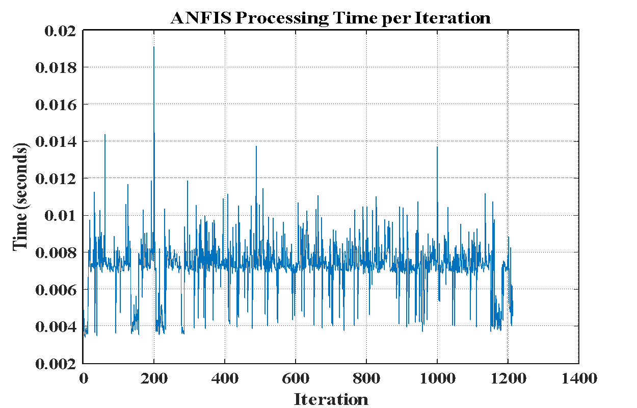
After observing the system's response, we evaluated the controller's computation time over approximately 1200 cycles for the system described in Fig. 18. The evaluation results were highly positive, indicating that the controller can operate effectively under real-time conditions, with its computation time being consistently faster than the sampling period (0.01 s). This serves as a foundation for further implementation on the physical model.

18. ANFIS processing time per iteration

5. Conclusion

In this study, we propose using MATLAB's ANFIS toolbox to learn from a controller that has been successfully simulated. A research paper on the mathematical modeling of this system and the implementation of LQR is being written simultaneously. Building on these successes, we have successfully applied an intelligent ANFIS controller in a simulation environment for a highly nonlinear system such as the double inverted pendulum on a cart. Through this research, we found that ANFIS has effectively learned the operation of LQR, making it a highly attractive option in fields such as mobile robotics and other control system applications. Our next objective is to apply this ANFIS controller to a real-time system, and the results of this study will serve as a valuable reference for future research and development.

Acknowledgment

This paper belongs to project SV2025-95 funded by HCMUTE. We, authors, want to give thanks to that support.

References

1. K. H. Lundberg, T. W. Barton, “History of Inverted-pendulum Systems,” IFAC Proceedings, vol. 42, no. 24, pp. 131-135, 2010, https://doi.org/10.3182/20091021-3-JP-2009.00025.
2. M. R. Dastranj, A. A. Khoshmardan, H. Ebrahimi, P. S. Rad, “Design optimal Fractional PID Controller for Inverted Pendulum with Genetic Algorithm,” Majlesi Journal of Mechatronic Systems, vol. 2, no. 2, pp. 1-5, 2013, https://ms.majlesi.info/index.php/ms/article/view/77.
3. K. Chakraborty, J. Mahato, R. R. Mukherjee, “Tuning of PID Controller of Inverted Pendulum Using Genetic Algorithm,” International Journal of Electronics & Communication Technology, vol. 4, no. 1, pp. 183-186, 2013, https://www.iject.org/vol4/spl1/c0059.pdf.  
4. M. R. Dastranj, M. E. Khoshmardan, F. S. Sijani, Y. Ghezi, “Design of Optimal PID Controller Using Genetic Algorithm,” Australian Journal of Basic and Applied Sciences, vol. 5, no. 10, pp. 996-1001, 2011, https://www.ajbasweb.com/old/ajbas/2011/October-2011/996-1001.pdf.
5. J. Yi, N. Yubazaki, K. Hirota, “Stabilization control of series-type double inverted pendulum system using the SIRMs dynamically connected fuzzy inference model,” Artificial Intelligence in Engineering, vol. 15, no. 3, pp. 297-308, 2001, https://doi.org/10.1016/S0954-1810(01)00021-8.

6. S. K. Yadav, S. Sharma, N. Singh, “Optimal Control of Double Inverted Pendulum Using LQR Controller,” International Journal of Advanced Research in Computer Science and Software Engineering, vol. 2, no. 2, pp. 189-192, 2012, https://sigmaland.ir/wp-content/uploads/2022/06/Fardapaper-Optimal-Control-of-Double-Inverted-Pendulum-Using-LQR-Controller.pdf.
7. M. R. Nalavade, M. J. Bhagat, V. V. Patil, “Balancing Double Inverted Pendulum on A cart by Linearization Technique,” International Journal of Recent Technology and Engineering, vol. 3, no. 1, 2014, https://www.ijrte.org/wp-content/uploads/papers/v3i1/A1031033114.pdf.
8. M.-D. Tran et al, “Analysis of Linear and Intelligent Control for Balancing Pendubot System,” Journal of Fuzzy Systems and Control, vol. 3, no. 1, pp. 16-21, 2024, https://doi.org/10.59247/jfsc.v3i1.272.
9. I. Chawla, V. Chopra and A. Singla, "Robust LQR Based ANFIS Control of x-z Inverted Pendulum," 2019 Amity International Conference on Artificial Intelligence (AICAI), pp. 818-823, 2019, https://doi.org/10.1109/AICAI.2019.8701333.
10. J. J. Craig, “Introduction to Robotics Mechanics and Control,” 3rd edition-Pearson Education, 2005, https://www.changjiangcai.com/files/text-books/Introduction-to-Robotics-3rd-edition.pdf.

11. J. -S. R. Jang, "ANFIS: adaptive-network-based fuzzy inference system," IEEE Transactions on Systems, Man, and Cybernetics, vol. 23, no. 3, pp. 665-685, 1993, https://doi.org/10.1109/21.256541.
12. S. Qiang, Q. Zhou, X. Z. Gao and S. Yu, "ANFIS controller for double inverted pendulum," 2008 6th IEEE International Conference on Industrial Informatics, pp. 475-480, 2008, https://doi.org/10.1109/INDIN.2008.4618147.
13. V. Mohan and N. Singh, "Performance comparison of LQR and ANFIS controller for stabilizing double inverted pendulum system," 2013 IEEE International Conference on Signal Processing, Computing and Control (ISPCC), pp. 1-6, 2013, https://doi.org/10.1109/ISPCC.2013.6663452.
14. C.-H. Nguyen, “ANFIS-based LQR Control for Rotary Double Parallel Inverted Pendulum,” Journal of Fuzzy Systems and Control, vol. 2, no. 2, pp. 109-116, 2024, https://doi.org/10.59247/jfsc.v2i2.214.
15. Y. Singh, A. Kumar and R. Mitra, "Design of ANFIS controller based on fusion function for rotary inverted pendulum," 2012 International Conference on Advances in Power Conversion and Energy Technologies (APCET), pp. 1-5, 2012, https://doi.org/10.1109/APCET.2012.6302046.
16. N.-T.-S. Nguyen, “An Application of STM32F4-Embedded ANFIS-Fuzzy Controller for Tower Crane,” Journal of Fuzzy Systems and Control, vol. 2, no. 3, pp. 189-196, 2024, https://doi.org/10.59247/jfsc.v2i3.260.