Adaptive Sliding Mode Control with a Nonlinear Sliding Surface for DC-Bus Voltage Regulation
in a Renewable-Energy-Based DC Microgrid

Rudi Uswarman 1,*, Rifqi Firmansyah 2, Firmansyah Nur Budiman 3, Taufal Hidayat 4, Triawan Nugroho 5

1 Department of Electrical Engineering, Institut Teknologi Sumatera, Lampung, Indonesia

2 Department of Electrical Engineering, Universitas Negeri Surabaya, Surabaya, Indonesia

3 Department of Electrical Engineering, Universitas Islam Indonesia, Yogyakarta, Indonesia

4 Department of Electrical Engineering, Institut Teknologi Padang, Sumatera Barat, Indonesia

5 Department of Electrical and Computer Engineering, King Abdul Aziz University, Jeddah, Saudi Arabia

Email: 1 uswarman@el.itera.ac.id, 2 rifqifirmansyah@unesa.ac.id, 3 firmansyah.nur@uii.ac.id,
4 taufalhidayat4960@gmail.com, 5 twignyo@stu.kau.edu.sa

*Corresponding Author

Abstract—This study proposes an adaptive sliding mode control (ASMC) scheme incorporating a nonlinear sliding surface (NSS), denoted ASMC-NSS, for direct-current (DC)-bus voltage regulation in a renewable-energy-based DC microgrid. ASMC augments conventional sliding mode control (CSMC) through channel-wise switching-gain scheduling based on the integral absolute error (IAE), while the NSS introduces bounded, state-dependent scaling of the current-tracking surface. The gain schedule adjusts the switching authority as the accumulated tracking error crosses prescribed thresholds, whereas the NSS shapes the reaching dynamics to improve transient tracking and suppress overshoot. The controller is applied to a system integrating a wind turbine, a photovoltaic (PV) array, and battery energy storage. MATLAB/Simulink comparisons with CSMC and ASMC without the NSS show that ASMC-NSS reduces the current-tracking IAE by 90.5% and 87.3%, respectively, and achieves a current settling time of 0.054 s. It maintains the 500 V DC bus with a maximum overshoot of 0.28 V and a 0.02 s recovery time to the ±0.5 V band. Lyapunov analysis establishes asymptotic stability of the ideal inner current loops and uniform ultimate boundedness under bounded matched uncertainties.

Keywords—Adaptive Sliding Mode Control; Battery; DC Microgrid; Nonlinear Sliding Surface; Photovoltaic; Wind Turbine

1. Introduction

The installed capacity of renewable power generation—particularly photovoltaic (PV) and wind energy—continues to grow annually [1]. This upward trend has driven extensive research aimed at advancing renewable energy technologies, including improvements in power converter systems [2]-[4]. However, developing reliable power converters remains challenging due to the intermittent nature of these energy sources. PV systems cannot generate electricity at night because they depend on solar irradiance within the visible spectrum, while wind energy output is inherently unstable due to fluctuating wind speeds. To address these limitations, battery energy storage systems can be employed to supply power when PV and wind generation are insufficient to meet demand [5]. Moreover, batteries can store excess energy produced during periods of high generation, thereby improving overall system efficiency and reliability [6].

Prior research on microgrid regulation spans optimized classical and intelligent control architectures. A two-degree-of-freedom proportional–integral–derivative (PID) controller tuned through a hybrid dragonfly and pattern-search algorithm has been developed for multi-microgrid load-frequency regulation and evaluated against conventional proportional–integral (PI) and PID controllers [7]. In parallel, an online-trained neural-network architecture has been applied to a grid-connected hybrid AC/DC microgrid to coordinate renewable-source maximum-power-point tracking (MPPT) and grid power exchange under multiple MATLAB/Simulink test conditions [8].

Hybrid converter-control structures extend this line of work to power-flow coordination and DC-bus regulation. One configuration interconnects AC and DC microgrids through a modified unified interphase power controller, assigning fuzzy control to the line power converters and nonlinear-disturbance-observer-based multiple-surface sliding mode control (SMC) to the bus power converter [9]. A complementary approach employs a nonlinear-disturbance-observer-based DC-bus controller that avoids remote load and source-power measurements while suppressing transient voltage fluctuations in a hybrid AC/DC microgrid [10].

Predictive and finite-time nonlinear schemes further broaden the available design space. Model-predictive current-and-power control for the battery converter has been coordinated with model-predictive voltage-and-power control for the AC/DC interlinking converter, thereby smoothing renewable-power fluctuations while regulating the DC bus and grid power exchange [11]. Integral-terminal and fast-integral-terminal SMC have likewise been formulated for a hybrid AC/DC microgrid with renewable generation and hybrid energy storage; the centralized design regulates the AC- and DC-bus voltages in grid-connected and islanded operation and is supported by Lyapunov analysis and real-time hardware-in-the-loop validation [12].

Recent studies have extended sliding-mode-based control for converter-dominated microgrids through robust adaptive compensation of multiple disturbances [13], observerless backstepping disturbance rejection [14], event-triggered distributed control under imperfect sources [15], and adaptive fixed-time terminal control [16]. At the converter level, adaptive SMC has been applied to a boost converter supplying an unknown constant-power load [17], while an exact-feedback-linearization-based adaptive second-order SMC has been developed for DC–DC boost converters [18]. Complementary developments in reaching-law design and sliding-surface analysis are reported in [19]-[21]. Within DC-microgrid applications, nonlinear optimal trajectory-tracking control has been combined with a super-twisting algorithm to strengthen DC-bus voltage regulation under disturbances [22]. Collectively, these studies motivate a closer examination of adaptive and higher-order SMC structures for coordinated DC-bus regulation in converter-dominated microgrids.

Among adaptive higher-order approaches, one design applies second-order sliding-mode control in both grid-connected and islanded operation and introduces a third-order algorithm for islanded operation to improve chattering attenuation; its stability properties are established through formal analysis [23].

At the supervisory-control level, a decentralized hierarchical framework combines sliding-mode and fractional-order control elements to regulate power, voltage, current, and frequency in a wind/PV/fuel-cell microgrid subject to unbalanced and nonlinear loads; validation is conducted using offline MATLAB/Simulink simulations and an OPAL-RT real-time digital simulator [24]. By contrast, an islanded DC-bus regulation strategy integrates an adaptive observer, sliding-mode control, and fixed-frequency pulse width modulation (PWM) to address source, load, and parameter variations [25].

From a finite-time robustness perspective, second- and third-order sliding-mode controllers have been developed for a different microgrid architecture, with formal finite-time convergence established for the resulting closed loop [26]. Beyond higher-order SMC, an interfacing-converter study compares model predictive control (MPC), SMC, and PI control within its own plant model [27], whereas a grid-connected PV strategy combines reinforcement-learning-based MPPT with SMC current injection and benchmarks it against fuzzy-logic and incremental-conductance SMC [28]. These studies provide useful methodological benchmarks; however, their plant structures, control objectives, and test conditions differ from those adopted here.

This literature demonstrates the value of adaptive, higher-order, predictive, and learning-assisted control strategies. Nevertheless, three gaps remain relative to the present control objective: the reviewed methods do not jointly combine a bounded state-dependent sliding coefficient with an integral absolute error (IAE)-based gain schedule; they do not use nested baselines on the same plant to isolate the individual contributions of adaptive gain scheduling and the nonlinear sliding surface (NSS); and their stability derivations do not explicitly account for the sign change in the bidirectional battery-converter input coefficient. Table 1 summarizes this literature positioning.

Accordingly, the novelty of this study lies in the technically coordinated integration of the proposed components rather than in claiming that each component is independently new. The proposed ASMC-NSS framework combines a normalized nonlinear progress function that maintains a positive and bounded sliding coefficient, channel-wise IAE-based gain scheduling, a saturation boundary layer, and explicit sign-consistent control laws for the wind, PV, and bidirectional-battery converters within a unified averaged DC-microgrid model. This integration is further supported by a common Lyapunov analysis and nested identical-plant comparisons.

1. Comparison of related control approaches and the positioning of ASMC-NSS

Within this architecture, the NSS reshapes the current-tracking surface, while the IAE schedule adjusts the switching authority as the accumulated error crosses prescribed thresholds. Their incremental effects are isolated through the nested CSMC, ASMC, and ASMC-NSS baselines under identical plant, load, and generation conditions.

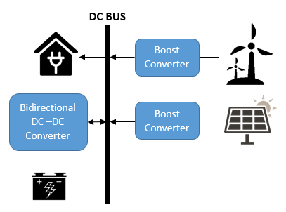
The controller is applied to an islanded renewable-energy-based DC microgrid that integrates PV and wind-turbine sources with battery storage, as illustrated in Fig. 1. Its performance is evaluated through matched MATLAB/Simulink simulations, while robustness is addressed analytically and within the explicitly stated operating-condition scope.

The main contributions of this study are summarized as follows:

• Development of a unified ASMC-NSS current-loop architecture for the wind-turbine, PV, and bidirectional-battery converters of an islanded DC microgrid.
• Formulation of a normalized and bounded NSS that preserves the equivalence Sᵢ = 0 ⇔ nᵢ = 0, together with explicit equivalent and complete control laws for the three converter channels.
• Development of channel-wise IAE-based gain scheduling that increases the switching authority when the accumulated tracking error exceeds predefined thresholds.
• Incorporation of a saturation boundary layer to attenuate discontinuous switching in the averaged current response.
• Establishment of a common Lyapunov stability analysis that explicitly accounts for the negative battery-channel input coefficient, followed by quantitative identical-plant comparisons of current tracking and 500-V DC-bus regulation using CSMC, ASMC, and ASMC-NSS.

1. Configuration of the DC microgrid

2. Modeling of the DC Microgrid

In the proposed configuration, wind and solar sources are coupled to a common DC bus through boost converters, while a battery is connected through a bidirectional converter. The model captures the dynamic behavior of each subsystem and expresses the complete microgrid in state-space form, thereby providing a structured basis for the controller design.

1. Modeling Assumptions

The analysis uses continuous-time averaged converter models operating in continuous-conduction mode. The DC bus is assumed to remain positive, and the wind, PV, and battery current references are bounded and piecewise differentiable. Throughout the controller derivation and the reported averaged-model simulations, ui ∈ ℝ denotes the unconstrained equivalent continuous control input of the ideal averaged model rather than the physical PWM duty ratio; no [0, 1] clipping is imposed on ui in the ideal stability derivation. Practical PWM mapping and actuator saturation are outside the present averaged-model scope. If imposed in a physical implementation, their matched residual is included in di(t) in (52) and must satisfy the robustness condition in (62). Converter conduction losses are represented by the series resistances Rw, Rpv, and Rbat; device-level PWM ripple, semiconductor switching loss, dead time, communication delay, and battery ageing are not explicitly modeled.

2. Dynamic Modeling of the Wind-Turbine System

A wind turbine converts mechanical motion into electrical energy. The dynamic behavior of the wind turbine is derived from the kinetic energy formulation, as expressed in (1) [33].

where  is the mechanical power (W),  is the rotor swept area (m²),  is the air density (kg/m³),  is the wind speed (m/s), and  is the turbine power coefficient, expressed as a function of the tip-speed ratio . The tip-speed ratio is

where  is the rotor angular velocity (rad/s) and  is the rotor radius (m). Substituting  from (2) into (1) gives,

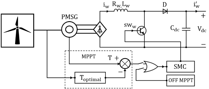
As shown in Fig. 2, the wind turbine drives a permanent-magnet synchronous generator (PMSG), whose output is rectified and delivered to the common DC bus through a boost converter comprising the input resistance and inductance, the controlled switch, the diode, and the DC-link capacitor. The supervisory logic selects either MPPT, which provides an optimal-torque-based reference, or off-MPPT operation, while the SMC generates the converter control action. This arrangement controls the wind-side current and the corresponding power transferred to the DC bus.

2. Configuration of the wind-turbine system

In this work, MPPT is achieved using the optimal torque control (OTC) method, which offers simplicity and high accuracy [34]. The technique modifies the PMSG torque for a given wind speed so that it matches the turbine’s maximum reference torque. Under the assumption of operation at the optimal tip-speed ratio and peak power coefficient,
 and  are replaced with  and . Hence, (3) can be expressed as:

Since , (4) can be rewritten as,

where  is the optimal torque reference. The wind-turbine current reference is then

where  is the DC output voltage of the uncontrolled rectifier. Acting as an equivalent load, the DC–DC boost converter regulates the PMSG rotational speed. Its averaged dynamics are

where , , , , , and  denote the wind-turbine output current, input inductance, DC-bus voltage, averaged converter control input, DC-link capacitance, and converter output current, respectively. Here,  and  denote the rectifier output voltage and the inductor series resistance, respectively.

3. Dynamic Modeling of the Photovoltaic System

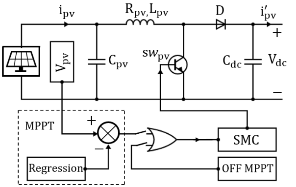
The PV energy system comprises a PV module and a boost converter. The high-level controller selects either MPPT or off-MPPT operation. The MPPT strategy uses a regression-plane model based on irradiance  (W/m²) and temperature  (°C) to compute the PV reference voltage  as follows [35]:

As shown in the configuration in Fig. 3, the PV energy system employs a boost converter. By applying averaged state modeling, the system's operational dynamics are derived and expressed through the differential equations provided below:

where , , , , , , , and  denote the PV-side current, PV voltage, input inductance, parasitic resistance, averaged converter control input, DC-bus voltage, DC-link capacitance, and converter output current, respectively.

3. Configuration of the PV system

1. Dynamic Modeling of the Battery System

The battery is connected to the DC bus through a bidirectional buck–boost converter that supports DC-bus regulation and controls battery charging and discharging according to the load and state of charge (SoC). Using the averaged converter model, the battery subsystem is described by (12)-(15). As illustrated in Fig. 4, the bidirectional battery converter provides separate switching paths for discharging (boost) and charging (buck) operation.

In the discharging (boost) mode, switch  is activated, whereas  operates as a diode. The battery then supplies energy to the DC bus, and the converter is described by,

where , , , and  denote the battery current, input inductance, boost-mode duty-ratio command, and converter output current, respectively. The symbols Vbat, Rbat, Vdc, and Cdc denote the battery terminal voltage, battery-side series resistance, DC-bus voltage, and DC-link capacitance, respectively.

4. Configuration of the battery system

In the charging (buck) mode, switch  is activated, whereas  operates as a diode. Here, u₂ denotes the buck-mode duty-ratio command. The converter model is

To obtain a unified model for both operating modes, define the virtual control input

where  is the operating-mode selector:  in discharging mode and  in charging mode. Substituting (16) into (12)-(15) gives the unified battery model

For reproducibility, the normalized battery state of charge  is obtained by coulomb counting. The sign convention is  during discharge and  during charge:

Here,  is the rated charge capacity, and  are the charge and discharge coulombic efficiencies. The reported short-duration simulation uses the ideal coulomb-counting case .

2. State-Space Model of the DC Microgrid

The hybrid microgrid, comprising the wind and PV sources, battery storage, and the DC load, is represented by the following state-space model.

Where , , and  are the wind, PV, and battery inductor currents, respectively, and  is the DC-bus voltage. The symbol Idc denotes the total current drawn by the DC load.

Expanding the control-input terms makes the control-affine structure explicit: ; ; . Here, ; ; .

The bus equation contains the input coefficients , , and . This expansion explains the positive wind/PV input coefficients and the negative battery-current input coefficient used in (36), (51), and (53).

1. Control Design for the DC Microgrid

The DC-microgrid controller combines conventional sliding mode control (CSMC), adaptive gain scheduling, and a nonlinear sliding surface. CSMC is first formulated for the wind-turbine, PV, and battery current loops. Gain scheduling then adjusts the available switching authority, whereas the NSS varies the sliding-surface scaling during the transient to accelerate tracking and reduce overshoot.

3. Conventional Sliding Mode Control

The conventional SMC design consists of a sliding surface, an equivalent control, and a switching control. The three current-loop sliding surfaces are defined as

where , , and  are the sliding surfaces for the wind-turbine, PV, and battery channels, respectively;  is the sliding coefficient; and  is the current-tracking error. The subscript d denotes the desired current reference for channel i. Differentiating the surfaces gives

Substituting , , and  from (20), (21), and (22) into (27), (28), and (29), respectively, gives

where , , and  are the equivalent controls for the wind-turbine, PV, and battery channels, respectively.

Setting  yields the equivalent controls

The switching component of SMC is defined as

where  is the switching gain,  is the unit saturation function,  is the boundary-layer thickness, and  is the input coefficient of channel . From (20)-(22), , , and .
The factor  therefore gives negative switching terms for the wind and PV channels and a positive switching term for the battery channel.

4. Adaptive Gain Scheduling for the Switching Control

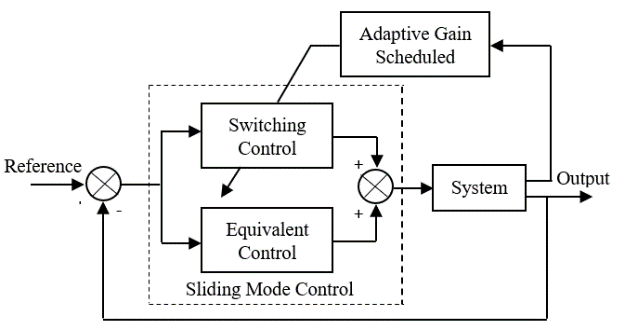
Adaptive SMC uses a channel-dependent switching gain  scheduled by the integral absolute error . The ASMC structure is shown in Fig. 5.

5. Adaptive SMC scheme

The gain is scheduled as,

The (40) schedules the gain as a nondecreasing function of the accumulated tracking error, with IAE expressed in A·s. A larger gain increases reaching authority and robustness, although an unnecessarily large value can increase control activity and sensitivity to measurement noise. Because cumulative IAE is nondecreasing, the gain cannot return to a lower level after a threshold is crossed. A moving-window IAE should therefore be used if downward gain adaptation is required after a transient.

5. Adaptive Control with a Nonlinear Sliding Surface

Motivated by prior NSS formulations [29]-[32], the nonlinear sliding surface is introduced as a bounded, state-dependent scaling of the current-tracking error. The shaping function is defined in (41).

Here,  is the nonlinear shaping function, and  sets its magnitude. The normalized progress variable is ; therefore, . The small constant  regularizes the denominator, and the absolute values make the normalization independent of the tracking direction. At the initial condition,  and ; as the current approaches its reference,  and . Consequently,  increases from  toward , modifying the sliding-surface scaling near the reference and helping to suppress overshoot. The three nonlinear sliding surfaces are

where  and  are design constants. The equivalent wind-turbine control is obtained by differentiating the nonlinear surface and imposing .

Substituting (20) into (46) gives the compact expression

where  is given by (20). Solving the equivalent-control condition in (47) gives

The complete wind-turbine ASMC-NSS law is

Using the baseline PV and battery equivalent controls in (34) and (35), respectively, the nonlinear equivalent and complete control laws are given in (50) and (51). The positive switching term in the battery law follows from the negative input coefficient in (22). In the simulations,
the common boundary-layer setting in Table 2 corresponds to ϑ₁ = ϑ₂ = ϑ₃ = ϑ.

2. System Parameters

6. Controller-Parameter Selection and Sensitivity

The controller parameters were selected subject to the analytical conditions in (55) and (62), followed by matched-condition tuning on the averaged model. The minimum surface coefficient is fixed by , whereas only the product  determines the range of . The redundant parameterization is therefore normalized by setting ; with  and , the implemented coefficient satisfies . If a different value of  is used,  should be rescaled so that .

The minimum switching gain must provide a positive robustness margin in (62). The levels  increase reaching authority as the channel IAE crosses 0.05 and 0.10 A·s. The (61) shows that a larger minimum gain shortens the boundary-layer reaching-time bound, while
(64)-(65) show that a smaller  tightens the ultimate error bound. These benefits are balanced against greater sensitivity to measurement noise and control activity; accordingly,  is used for all channels. The baseline coefficient  is held fixed across the CSMC comparison, and the same plant, references, and evaluation interval are used for every controller.

7. Lyapunov Stability Analysis

This subsection establishes the closed-loop stability of the proposed adaptive sliding-mode controller with a nonlinear sliding surface (ASMC-NSS). Let  denote the wind-turbine, PV, and battery current channels, respectively. From (20)-(22), their dynamics can be expressed in the compact form

where  is a lumped matched uncertainty representing parameter variations, unmodeled current-channel dynamics, external disturbances, practical actuator-saturation residuals, and derivative-estimation errors. The input coefficients associated with the three converter models are,

The negative sign of  is essential: the stabilizing switching term of the battery controller must have the opposite sign to those of the wind and PV controllers, as implemented in (51). The analysis assumes that , so that ; the reference currents  and their derivatives are bounded. No [0, 1] bound is imposed on the ideal continuous control input; practical actuator saturation, if imposed, is treated through the matched residual in (52).

Define the tracking error, nonlinear coefficient, and nonlinear sliding variable as.

Because the progress variable in (41) is saturated to , the nonlinear function satisfies . Therefore, for , , and ,

Consequently,  is equivalent to . The finite positive parameter  determines , whereas the small constant  in (41) only regularizes the denominator used to construct  and does not alter the Lyapunov inequalities. Because  prevents a singular denominator and  is constructed using absolute-value and saturation operations,  is locally absolutely continuous on every interval over which  and  are locally absolutely continuous. Consequently, the composite shaping function  is differentiable almost everywhere, and its time derivative in (45)-(58) is understood in the almost-everywhere sense on intervals between reference discontinuities. At an isolated reference jump, the analysis is applied piecewise on the adjacent continuous intervals.

Since  and  are constants, the correct derivative of the nonlinear surface is,

The (56) includes (45) as the wind-turbine case. In particular, the second term is . Using the compact notation in (52), the equivalent and complete control laws can be written as,

For , (57) gives a negative switching component; for , it gives a positive component. Substituting (57) into (52) and then into (56) yields,

Theorem 1 (ideal averaged model). Suppose that ,  satisfies (55), , and . Then the equilibrium  is asymptotically stable, and all three current-tracking errors converge to zero.

Proof. Consider the following common quadratic Lyapunov candidate:

The summation in (59) is appropriate because it combines the three scalar Lyapunov functions of the wind, PV, and battery current loops. It is positive definite with respect to . Along the ideal closed-loop trajectories,

For every , the product  is positive: it equals  outside the boundary layer and  inside it. Since , , and , (60) gives  for  and  only at . Hence, the origin of the sliding-variable dynamics is asymptotically stable. Because  and ,  for .

Outside the boundary layer, the saturation function becomes . An upper bound on the time required to reach  is,

with an ideal sign function,  and (61) becomes a finite-time reaching bound for . With the saturation function used in this study, the ideal dynamics are exponentially convergent inside the boundary layer.

Theorem 2 (bounded matched uncertainties). Suppose that  and that the minimum switching gain satisfies

Then every sliding variable reaches the prescribed boundary layer in finite time and the current-tracking errors are uniformly ultimately bounded.

Proof. From (58), outside the boundary layer,

Inside the boundary layer, completing the scalar inequality for each channel gives the conservative bounds

and, because ,

Thus, a smaller boundary-layer thickness improves the theoretical tracking-error bound but increases sensitivity to chattering and sampling effects. Actuator saturation remains admissible only when its residual is included in  and condition (62) is preserved.

The scheduled gains in (40) satisfy Aᵢ(t)∈{90,110,130}, so Aᵢ,min=90>0. The Lyapunov function in (59) is therefore common to all three gain levels, and no Aᵢ term appears because Aᵢ is not included as a Lyapunov state. Switching between gain levels does not invalidate the proof provided that (62) holds. The schedule in (40) is nondecreasing with cumulative IAE rather than continuously proportional to it. A moving-window IAE should be used if the gain is intended to decrease again after a transient.

Finally, (59)-(65) prove stability of the three inner current-tracking loops; they do not independently prove convergence of the fourth state . Let . If the outer reference-current generator is designed so that the nominal bus-current balance produces , , then (23) can be written as

For ,

Therefore, the DC-bus subsystem is input-to-state stable with respect to the inner-loop current mismatch. If Theorem 1 applies and the continuous averaged-model control inputs ), ), and ) remain bounded along the closed-loop trajectories, then )→0 implies →0 through (67), and (68) consequently gives )→0. This bounded-signal requirement is a closed-loop regularity assumption needed for the product terms in ; it is not a hard amplitude constraint on the control variable. Thus,  is not restricted to [0,1] and remains an unconstrained continuous input of the averaged model. Under the conditions of Theorem 2, the DC-bus voltage is uniformly ultimately bounded. Without an explicitly defined outer-loop law satisfying (66)-(67), the formal Lyapunov claim must be limited to the three converter current-tracking loops, while DC-bus regulation is supported by the simulation results.

For the first-order current channels considered here,  is most rigorously interpreted as a state-dependent scaling of the sliding surface that modifies the reaching dynamics and control effort. A literal damping-ratio interpretation requires an explicitly defined second-order reduced error model; the stability conclusions above do not rely on that interpretation.

2. Results and Discussion

1. Simulation Scope and Operating Conditions

The simulations were performed in MATLAB/Simulink over a common 0–13 s interval using the fixed-step ode3 (Bogacki–Shampine) solver with a fixed-step size of 1 × 10⁻⁴ s. The discrete base rate and nominal converter switching frequency were both set to 10 kHz, corresponding to a base-rate sample time of 1 × 10⁻⁴ s. Because the converter plant is represented by the continuous-time averaged (7)-(23), individual PWM pulses and semiconductor switching ripple at the nominal 10-kHz carrier frequency are not explicitly resolved; the switching frequency is reported as an implementation parameter. The simulation starts at t = 0 s, when the prescribed source, load, and current-reference profiles are applied. The DC-bus reference is 500 V, and the normalized battery SoC is initialized at 1.0 p.u. All controllers use identical plant parameters, reference trajectories, load events, numerical settings, and metric definitions.

The matched comparison includes the reported load-resistance, wind-speed, and temperature profiles, while irradiance is fixed at 900 W/m². The series resistances in Table 2 represent fixed nominal conduction-loss terms rather than a converter-loss sensitivity study. The expanded campaign suggested by the reviewer—irradiance variation, a wider wind-speed range, additional sudden load changes, parameter uncertainty, detailed converter-loss variation, and sensor noise—was not performed in this revision and is reserved for future work. No numerical result is claimed for these unperformed cases.

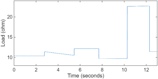
The DC microgrid is simulated in MATLAB/Simulink using the parameters and configuration summarized in
Table 2. The load, wind-speed, and temperature profiles used for the matched controller comparison are shown in
Fig. 6 to Fig. 8, respectively.

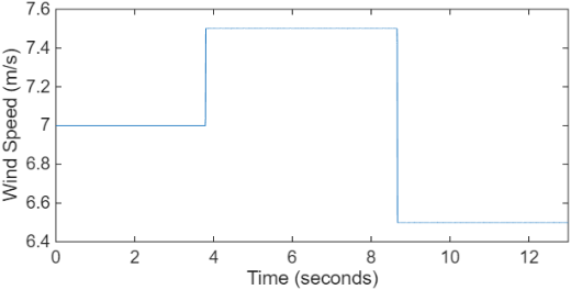
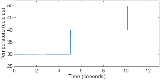
As illustrated in Fig. 6, the load resistance begins at 10.4 Ω and changes abruptly up to 22.7 Ω. Fig. 7 shows wind-speed steps among 7.0, 7.5, and 6.5 m/s. The PV irradiance is held at 900 W/m², while the temperature follows the profile in Fig. 8.

6. Load profile

7. Wind-speed profile

8. Temperature profile

1. Quantitative Performance

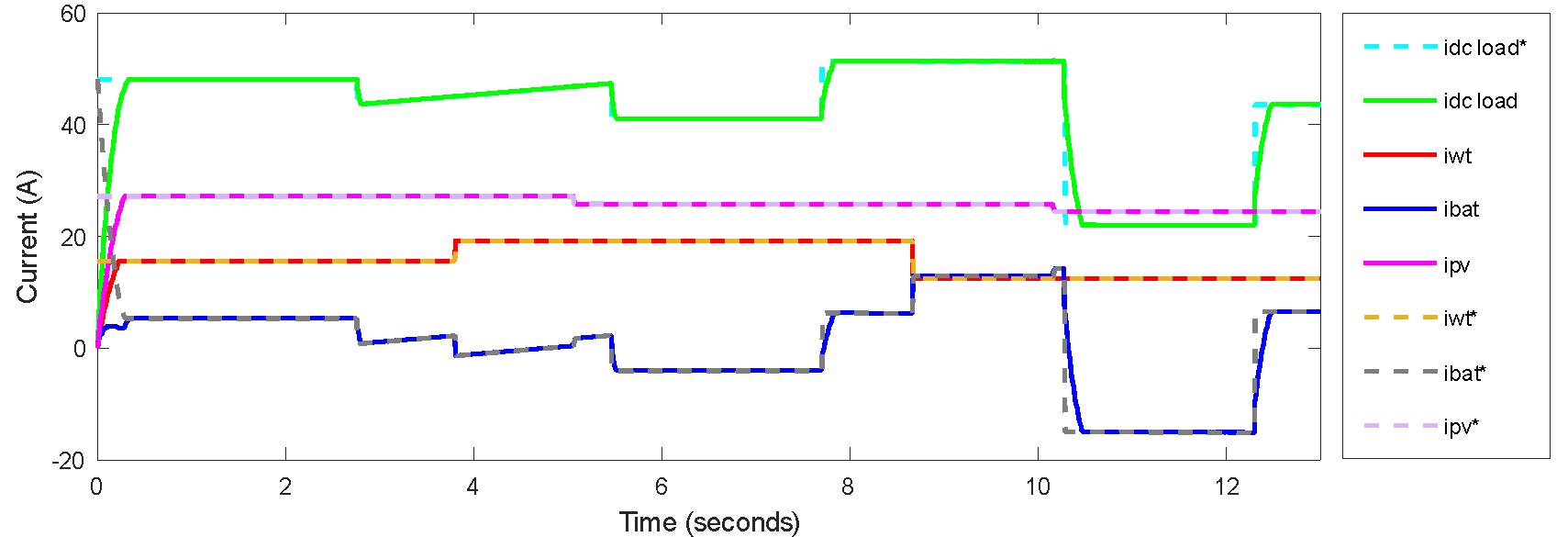
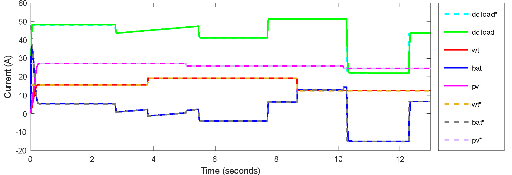
The performance of the wind-turbine, photovoltaic (PV), and battery current loops is evaluated for three control strategies, as illustrated in Fig. 9 to Fig. 11. All three controllers distribute power to meet the DC-load demand, but their tracking responses differ. CSMC uses fixed switching gains and exhibits less precise tracking and more visible high-frequency variation in Fig. 9. The ASMC response in Fig. 10 benefits from gain scheduling as the accumulated tracking error crosses the prescribed thresholds. ASMC-NSS provides the closest agreement between measured and reference currents in Fig. 11 under the simulated generation and load variations.

Fig. 12 compares the output-current transients obtained with CSMC, ASMC, and the proposed ASMC-NSS under identical load changes. The quantitative indices in Table 3 use the same simulation interval for all controllers. IAE represents the accumulated error magnitude, whereas RMSE gives greater weight to larger instantaneous errors; therefore, reductions in both indices indicate improved tracking over the complete transient rather than only at a single operating point.

The current-overshoot entries in Table 3 are dimensionless ratios and are therefore reported in per unit (p.u.). Percentage reduction is calculated as 100 × (baseline − ASMC-NSS)/baseline using the reported values and is rounded to one decimal place.

3. Quantitative current-tracking performance based on Fig. 12

Relative to CSMC, conventional ASMC lowers the current-tracking IAE by 25.5% and the RMSE by 10.3%. The addition of the NSS produces a substantially larger improvement: ASMC-NSS reduces IAE by 90.5% and RMSE by 72.2% against CSMC, and by 87.3% and 69.0%, respectively, against ASMC, as shown in Table 4. The rise time decreases from 0.370 s (CSMC) and 0.280 s (ASMC) to 0.031 s, corresponding to reductions of 91.6% and 88.9%. Likewise, the 0.054-s settling time is 89.4% shorter than CSMC and 85.4% shorter than ASMC, while the overshoot magnitude is reduced by 97.6% and 84.4%. These simultaneous improvements are consistent with the NSS varying the effective sliding-surface scaling during the transient, thereby accelerating reaching while suppressing the tracking error near the reference.

The saturation boundary layer attenuates discontinuous switching in the averaged current response, but the manuscript does not claim complete chattering elimination. A controller-output total-variation index would be strongly dependent on solver resolution in an averaged model and would not quantify semiconductor switching ripple. Chattering is therefore interpreted together with the current RMSE, overshoot, and plotted high-frequency variation under the same numerical settings. Device-level PWM simulations or experiments that report control-signal total variation and switching loss are identified as future work.

4. Current-tracking error reduction achieved by ASMC-NSS

Fig. 13 evaluates voltage regulation around the 500 V reference. Table 5 summarizes the maximum overshoot, recovery time, IAE, and RMSE for the three controllers, while Table 6 reports the reduction obtained by ASMC-NSS relative to each baseline.

ASMC-NSS limits the maximum DC-bus overshoot to 0.28 V, which is 20.0% lower than CSMC and 17.6% lower than ASMC. Its 0.02-s recovery time is 88.9% shorter than CSMC and 85.7% shorter than ASMC. The IAE decreases to 1.69 V·s, giving reductions of 19.9% and 19.1%, whereas the RMSE decreases to 0.14 V, corresponding to reductions of 26.3% and 22.2%. The smaller percentage gains at the DC bus than in the current loops are expected because the DC-link capacitor buffers short-duration current imbalance and all three controllers already maintain a small absolute voltage error. Nevertheless, the consistently lower overshoot, recovery time, IAE, and RMSE show that the improved current tracking is translated into tighter DC-bus regulation.

5. Quantitative DC-bus voltage performance based on Fig. 13

For the 500 V reference, ±0.5 V corresponds to a ±0.1% band. The reported value is therefore interpreted as recovery time to this tight band, rather than the conventional 10–90% rise time.

6. DC-bus error reduction achieved by ASMC-NSS

Finally, Fig. 14 shows the normalized battery SoC. Under the sign convention in (19), positive battery current decreases SoC during discharge, whereas negative current increases SoC during charging. The small excursion from approximately 1.0 p.u. is consistent with the 34-Ah capacity and the short 13 s simulation interval. Because battery ageing and electrochemical stress are not modeled, the figure is interpreted as an energy-balance indicator rather than evidence of degradation reduction.

The results from Fig. 9 to Fig. 14 and Table 3 to Table 6 confirm that the proposed ASMC-NSS improves both converter-current tracking and DC-bus voltage regulation. Relative to CSMC and ASMC, respectively, current-tracking IAE is reduced by 90.5% and 87.3%, while DC-bus IAE is reduced by 19.9% and 19.1%. The agreement among IAE, RMSE, rise/recovery time, settling time, and overshoot metrics supports the conclusion that the performance gain is not confined to a single index.

Theorem 2 establishes boundedness under matched uncertainty, but this analytical result does not replace numerical validation under the broader conditions suggested by the reviewer. Future work will therefore examine irradiance variation, a wider wind-speed range, additional load-step scenarios, coordinated parameter uncertainty, detailed converter-loss variation, and sensor noise using a common plant model, controller settings, and evaluation protocol.

The numerical comparison deliberately uses CSMC and ASMC as nested baselines on the identical plant so that the incremental effects of adaptive gain scheduling and the nonlinear surface can be isolated. Direct numerical values from MPC, PI/PID, higher-order SMC, fuzzy-SMC, or RL-SMC studies are not combined with Table 3 to Table 6 because those studies use different converter topologies, objectives, constraints, sampling rates, and disturbance profiles. Table 1 provides a literature-based positioning instead; a matched-plant benchmark against one representative advanced controller is reserved for
future work.

9. Output currents using CSMC

10. Output currents using ASMC

11. Output currents using ASMC-NSS

12. Comparison of output-current responses

13. DC-bus voltage comparison

14. Normalized battery SoC (p.u.; 1.0 p.u. = 100%)

3. Conclusion

This study developed an ASMC-NSS controller for the power converters of an islanded DC microgrid. The adaptive gain schedule maintains switching authority as the tracking error changes, while the NSS provides a bounded state-dependent scaling of the sliding surface to improve the transient response. The Lyapunov analysis establishes asymptotic stability of the ideal inner current loops and uniform ultimate boundedness in the presence of bounded matched uncertainties; the DC-bus result is interpreted through the stated outer-loop assumption.

Under the reported matched MATLAB/Simulink conditions, ASMC-NSS produces lower current-tracking and DC-bus error metrics than CSMC and standard ASMC. Current-tracking IAE is reduced by 90.5% relative to CSMC and by 87.3% relative to ASMC, while the corresponding DC-bus IAE reductions are 19.9% and 19.1%. The proposed controller achieves a 0.054-s current settling time, limits the maximum DC-bus overshoot to 0.28 V, and returns the 500 V bus to the ±0.5 V band within 0.02 s.

Future work will extend the validation to irradiance variation, a wider wind-speed range, additional sudden load changes, coordinated parameter uncertainty, detailed converter-loss models, and sensor noise. These cases will be evaluated through a controlled simulation campaign using identical controller settings and metric definitions. Hardware-in-the-loop and prototype experiments will subsequently report control-signal total variation and switching loss. A matched-plant benchmark against one representative advanced controller, such as MPC or higher-order SMC, will be used to avoid an unstructured comparison across incompatible models. Multi-objective tuning of β, φ, ϑᵢ, and the adaptive-gain thresholds will target shorter settling and recovery times, smaller DC-bus deviation and overshoot, and lower current IAE and RMSE. An explicit outer DC-bus controller will also be developed to extend the inner-loop Lyapunov result to the complete closed loop.

References

1. H. Tiismus, V. Maask, V. Astapov, T. Korotko, and A. Rosin, “State-of-the-Art Review of Emerging Trends in Renewable Energy Generation Technologies,” IEEE Access, vol. 13, pp. 10820–10843, 2025, https://doi.org/10.1109/ACCESS.2025.3528640.
2. V. Yadav, A. Chub, and N. Yadav, “Reconfigurable Non-Isolated DC-DC Converter for DC Microgrid Applications,” IEEE Open Journal of Power Electronics, vol. 7, pp. 425–438, 2026, https://doi.org/10.1109/OJPEL.2026.3655650.
3. V. F. Pires, A. Cordeiro, D. Foito, J. Monteiro, and A. J. Pires, “Bidirectional DC-DC Converter with High Voltage Step-Up/Down Ratio and Voltage Balance Capability for the Interconnection of Unipolar and Bipolar DC Microgrids,” IEEE Transactions on Industry Applications, 2026, https://doi.org/10.1109/TIA.2026.3655649.
4. V. Fernao Pires, D. Foito, A. Cordeiro, P. Pereira, and J. Martins, “A Single-Switch DC-DC Nonisolated Boost and Buck-Boost Converters with Wide Voltage Gain for Unipolar and Bipolar DC Microgrids,” IEEE Open Journal of Power Electronics, vol. 7, pp. 570–585, 2026, https://doi.org/10.1109/OJPEL.2026.3655438.
5. N. B. Kampa, S. Vuddanti, and S. V. K. Naresh, “A Novel Model Predictive Control-Based Energy Management for Stable and Efficient Operation of Renewable Integrated DC Microgrids,” IEEE Access, vol. 14, pp. 49413–49427, 2026, https://doi.org/10.1109/ACCESS.2026.3678042.

6. N. Yadav, A. Chub, T. Mitra, and A. Makkieh, “Fault Scenarios and Protection Challenges in Multiport Partial Power Converters for PV-Battery Integrated DC Microgrids,” IEEE Open Journal of Power Electronics, vol. 7, pp. 749–758, 2026, https://doi.org/10.1109/OJPEL.2026.3661119.
7. S. Mishra, R. C. Prusty, and S. Panda, “Design and Analysis of 2dof-PID Controller for Frequency Regulation of Multi-Microgrid Using Hybrid Dragonfly and Pattern Search Algorithm,” Journal of Control, Automation and Electrical Systems, vol. 31, no. 3, pp. 813–827, 2020, https://doi.org/10.1007/s40313-019-00562-y.
8. N. Chettibi, A. Mellit, G. Sulligoi, and A. Massi Pavan, “Adaptive Neural Network-Based Control of a Hybrid AC/DC Microgrid,” IEEE Transactions on Smart Grid, vol. 9, no. 3, pp. 1667–1679, 2018, https://doi.org/10.1109/TSG.2016.2597006.
9. M. Zolfaghari, M. Abedi, and G. B. Gharehpetian, “Power Flow Control of Interconnected AC-DC Microgrids in Grid-Connected Hybrid Microgrids Using Modified UIPC,” IEEE Transactions on Smart Grid, vol. 10, no. 6, pp. 6298–6307, 2019, https://doi.org/10.1109/TSG.2019.2901193.
10. C. Wang, X. Li, L. Guo, and Y. W. Li, “A nonlinear-disturbance-observer-based DC-Bus voltage control for a hybrid AC/DC microgrid,” IEEE Transactions on Power Electronics, vol. 29, no. 11, pp. 6162–6177, 2014, https://doi.org/10.1109/TPEL.2013.2297376.

11. Y. Shan, J. Hu, K. W. Chan, Q. Fu, and J. M. Guerrero, “Model Predictive Control of Bidirectional DC-DC Converters and AC/DC Interlinking Converters-A New Control Method for PV-Wind-Battery Microgrids,” IEEE Transactions on Sustainable Energy, vol. 10, no. 4, pp. 1823–1833, 2019, https://doi.org/10.1109/TSTE.2018.2873390.
12. H. Armghan, M. Yang, A. Armghan, N. Ali, M. Q. Wang, and I. Ahmad, “Design of integral terminal sliding mode controller for the hybrid AC/DC microgrids involving renewables and energy storage systems,” International Journal of Electrical Power and Energy Systems, vol. 119, 2020, https://doi.org/10.1016/j.ijepes.2020.105857.
13. L. Liu et al., “Multidisturbances Compensation for Three-Level NPC Converters in Microgrids: A Robust Adaptive Sliding Mode Control Approach,” IEEE Transactions on Industrial Informatics, vol. 20, no. 6, pp. 8917–8931, 2024, https://doi.org/10.1109/TII.2024.3370237.
14. A. Chabukswar and R. Wandhare, “Modified Back-Stepping Sliding Mode Controller with Robust Observer-Less Disturbance Rejection for DC Microgrid Applications,” IEEE Transactions on Power Electronics, vol. 40, no. 1, pp. 451–466, 2025, https://doi.org/10.1109/TPEL.2024.3462448.
15. L. Liu, Y. Wang, Z. Zhang, and Z. Zuo, “Event-Triggered Distributed Sliding Mode Control for DC Microgrids With Imperfect Sources,” IEEE Transactions on Industrial Informatics, vol. 21, no. 1, pp. 435–444, 2025, https://doi.org/10.1109/TII.2024.3452686.

16. A. Chabukswar and R. Wandhare, “Adaptive Feedforward Sliding Curve-Based Hybrid Fixed-Time Extended-Order Terminal Sliding-Mode Control for DC Microgrids,” IEEE Journal of Emerging and Selected Topics in Industrial Electronics, vol. 6, no. 2, pp. 719–730, 2025, https://doi.org/10.1109/JESTIE.2024.3517713.
17. D. A. Zambrano-Prada, A. El Aroudi, O. Lopez-Santos, L. Vazquez-Seisdedos, and L. Marti-Nez-Salamero, “Adaptive Sliding Mode Control of a Boost Converter with Unknown Constant Power Load,” IEEE Access, vol. 13, pp. 33714–33732, 2025, https://doi.org/10.1109/ACCESS.2025.3543659.
18. J. Sun, J. Xia, S. Ding, and X. Yu, “Exact-Feedback-Linearization-Based Adaptive Second-Order Sliding Mode Control Design for DC–DC Boost Converters,” IEEE Transactions on Industrial Electronics, vol. 72, no. 5, pp. 5397–5407, 2025, https://doi.org/10.1109/TIE.2024.3476994.

19. Y. Wang, Y. Feng, X. Zhang, and J. Liang, “A New Reaching Law for Antidisturbance Sliding-Mode Control of PMSM Speed Regulation System,” IEEE Transactions on Power Electronics, vol. 35, no. 4, pp. 4117–4126, 2020, https://doi.org/10.1109/TPEL.2019.2933613.

20. Y. Su, “Comments on ‘A New Adaptive Sliding-Mode Control Scheme for Application to Robot Manipulators,’” IEEE Transactions on Industrial Electronics, vol. 67, no. 8, pp. 7116–7120, 2020, https://doi.org/10.1109/TIE.2019.2939995.
21. Y. Zhang, Q. Zhang, J. Zhang, and Y. Wang, “Sliding Mode Control for Fuzzy Singular Systems with Time Delay Based on Vector Integral Sliding Mode Surface,” IEEE Transactions on Fuzzy Systems, vol. 28, no. 4, pp. 768–782, 2020, https://doi.org/10.1109/TFUZZ.2019.2916049.
22. F. Ornelas-Tellez, J. J. Rico-Melgoza, E. Espinosa-Juarez, and E. N. Sanchez, “Optimal and robust control in DC microgrids,” IEEE Transactions on Smart Grid, vol. 9, no. 6, pp. 5543–5553, 2018, https://doi.org/10.1109/TSG.2017.2690566.
23. Y. Han, R. Ma, and J. Cui, “Adaptive higher-order sliding mode control for islanding and grid-connected operation of a microgrid,” Energies, vol. 11, no. 6, p. 1459, 2018, https://doi.org/10.3390/en11061459.
24. H. R. Baghaee, M. Mirsalim, G. B. Gharehpetian, and H. A. Talebi, “Decentralized Sliding Mode Control of WG/PV/FC Microgrids under Unbalanced and Nonlinear Load Conditions for On- and Off-Grid Modes,” IEEE Systems Journal, vol. 12, no. 4, pp. 3108–3119, 2018, https://doi.org/10.1109/JSYST.2017.2761792.
25. D. Zhang and J. Wang, “Adaptive Sliding-Mode Control in Bus Voltage for an Islanded DC Microgrid,” Mathematical Problems in Engineering, vol. 2017, p. 8962086, 2017, https://doi.org/10.1155/2017/8962086.

26. M. Cucuzzella, G. P. Incremona, and A. Ferrara, “Design of Robust Higher Order Sliding Mode Control for Microgrids,” IEEE Journal on Emerging and Selected Topics in Circuits and Systems, vol. 5, no. 3, pp. 393–401, 2015, https://doi.org/10.1109/JETCAS.2015.2450411.
27. S. K. Panda and A. Ghosh, “A Computational Analysis of Interfacing Converters with Advanced Control Methodologies for Microgrid Application,” Technology and Economics of Smart Grids and Sustainable Energy, vol. 5, no. 1, 2020, https://doi.org/10.1007/s40866-020-0077-x.
28. A. Bag, B. Subudhi, and P. K. Ray, “A combined reinforcement learning and sliding mode control scheme for grid integration of a PV System,” CSEE Journal of Power and Energy Systems, vol. 5, no. 4, pp. 498–506, 2019, https://doi.org/10.17775/cseejpes.2017.01000.
29. A. E. K. Mohammad, N. Uchiyama, and S. Sano, “Reduction of electrical energy consumed by feed-drive systems using sliding-mode control with a nonlinear sliding surface,” IEEE Transactions on Industrial Electronics, vol. 61, no. 6, pp. 2875–2882, 2014, https://doi.org/10.1109/TIE.2013.2275975.
30. A. E. K. Abd El, N. Uchiyama, and S. Sano, “Energy saving in feed drive systems using sliding-mode-based contouring control with a nonlinear sliding surface,” IEEE/ASME Transactions on Mechatronics, vol. 20, no. 2, pp. 572–579, 2015, https://doi.org/10.1109/TMECH.2013.2296698.

31. B. Bandyopadhyay and D. Fulwani, “High-performance tracking controller for discrete plant using nonlinear sliding surface,” IEEE Transactions on Industrial Electronics, vol. 56, no. 9, pp. 3628–3637, 2009, https://doi.org/10.1109/TIE.2008.2007984.
32. D. Fulwani, B. Bandyopadhyay, and L. Fridman, “Non-linear sliding surface: Towards high performance robust control,” IET Control Theory and Applications, vol. 6, no. 2, pp. 235–242, 2012, https://doi.org/10.1049/iet-cta.2010.0727.
33. H. Armghan, M. Yang, M. Q. Wang, N. Ali, and A. Armghan, “Nonlinear integral backstepping based control of a DC microgrid with renewable generation and energy storage systems,” International Journal of Electrical Power and Energy Systems, vol. 117, p. 105613, 2020, https://doi.org/10.1016/j.ijepes.2019.105613.
34. M. A. Abdullah, A. H. M. Yatim, C. W. Tan, and R. Saidur, “A review of maximum power point tracking algorithms for wind energy systems,” Renewable and Sustainable Energy Reviews, vol. 16, no. 5, pp. 3220–3227, 2012, https://doi.org/10.1016/j.rser.2012.02.016.
35. Naghmash, H. Armghan, I. Ahmad, A. Armghan, S. Khan, and M. Arsalan, “Backstepping based non-linear control for maximum power point tracking in photovoltaic system,” Solar Energy, vol. 159, pp. 134–141, 2018, https://doi.org/10.1016/j.solener.2017.10.062.