Journal of Fuzzy Systems and Control, Vol. 4, No 2, 2026 |
|
A Multi-Channel Wavelet Long Short-Term Memory Framework for Early Wheel Slip
Detection in Urban Light Rail Transit
Yulian Lingga Permana 1, Muhammad Hamka Ibrahim 2,*, Hari Maghfiroh 3
1, 2, 3 Department of Electrical Engineering, Universitas Sebelas Maret, Surakarta, Indonesia
Email: 1 lingga.permana@student.uns.ac.id, 2 hamka@staff.uns.ac.id, 3 hari.maghfiroh@staff.uns.ac.id
*Corresponding Author
Abstract—This paper presents an integrated framework combining Continuous Wavelet Transform (CWT) with multi-stream Long Short-Term Memory and Multi-Layer Perceptron (LSTM+MLP) networks for early wheel slip detection in urban Light Rail Transit (LRT). Conventional Wheel Slip Protection (WSP) systems rely on static thresholds applied to axle speed differences, resulting in detection latency that impacts wheel-rail wear and operational disruptions. Three methodological contributions are proposed: (i) a five-channel CWT feature extraction strategy that leverages the structural hierarchy of LRT trainsets consisting of motor car with cabin (MC), motor car (M), and trailer car (T); (ii) a conventional ground truth labeling workflow using Slip/Slide Status signals as a reference, eliminating expert annotation bias; and (iii) the first distance-based spatial slip hotspot mapping integrated with model prediction for the Jakarta LRT line. The framework is validated on a 50-minute operational dataset consisting of 93,755 time steps with a resolution of 32 ms, collected from the LRT and synchronized via Dynamic Time Warping using 47 Train Control and Management System (TCMS) variables with three different sampling rates. Statistical analysis confirms that the motor-trailer speed difference channel achieves a Cohen's d of 1.615 with a Kolmogorov-Smirnov p < 0.001 test between normal and slip distributions. The integrated LSTM+MLP model achieves an F1 score of 0.9272, an AUC of 0.9958, and a median early detection margin of 1.152 seconds before conventional WSP activation, with 100% of test events detected earlier than the conventional system. Complementary spatial mapping derived from a larger multi-train dataset containing 5,948 events identified 414 high-risk zones along the LRT track, supporting predictive WSP threshold modulation and maintenance scheduling that takes rail wear into account.
Keywords—Continuous Wavelet Transform; Deep Learning; Light Rail Transit; Long Short-Term Memory; Predictive Maintenance; Wheel Slip Detection
Nomenclature
Symbol | Meaning | Unit/domain |

| Continuous and discretised time | s / index |

| Sampling interval (= 0.032 s) | s |

| Samples of the reference and target sequence for DTW | km/h |
 , , 
| Local and cumulative DTW cost (L₂) | (km/h)² |

| Optimal DTW alignment path | index sequence |

| Five-channel input signals (Table 4) | km/h, bar, – |

| Angular gradient of a channel | rad |

| Sample lag for the angular gradient (= 8) | samples |

| Morlet mother wavelet scaled by α | dimensionless |

| Wavelet scale, α ∈ [1, 128] | dimensionless |

| CWT coefficient at scale α and time t | |·| dimensionless |

| Per-time-step feature vector | real |

| Per-window LSTM input tensor | real |

| LSTM forget / input/output gates | [0,1] |

| LSTM cell state and hidden output | real |

| Dense pre-activation logit and ReLU activation | real |

| Sigmoid output, P(slip | window) | [0,1] |

| Classification threshold (= 0.158) | [0,1] |

| Onset time of conventional WSP and model | s |

| Early-detection margin = tₚₗc − tₗₛₜₘ | s |

| Event count and heavy-slip count in a 50-m zone | count |

| Total slip duration in the zone | s |

| Geometric factor (0 = flat, 1 = curve or grade, 2 = both) | [0, 2] |

| Composite zone-priority score | real |
Introduction
Wheel slip originates in the nonlinear creep behaviour of the wheel–rail contact, where the tangential force saturates as creepage grows [1], and its repeated occurrence contributes to accelerated wheel–rail wear, rolling contact fatigue, and reduced ride quality [2]. In urban Light Rail Transit (LRT) systems, where frequent acceleration-braking cycles occur between adjacent stations, the cumulative effect of undetected micro-slip events can substantially shorten rolling stock wheel life and increase maintenance and life-cycle costs [3]. Mei and Chen [4] showed that on track curvatures with a radius below 350 m, rail corrugation caused by wheel slippage occurred in almost all observed cases, directly linking slip detection capability to infrastructure longevity.
Modern railway systems generally use WSP systems based on conventional threshold logic applied to the difference in shaft speeds [5]. Although these systems operate reliably under severe slippage conditions, they have two major limitations: (i) unavoidable detection latency, since the protection mechanism can only be activated after a predetermined threshold is exceeded [6]; and (ii) a lack of sensitivity to low-amplitude micro-slip events, which, although small in scale, cumulatively contribute to wheel-rail wear over the long term [7]. This gap has spurred an increasing number of studies on data-driven displacement detection, in which operational sensor data replaces static thresholds as the primary input for decision-making, thereby enabling early signs of slip to be identified before the conventional WSP is activated.
Pioneering research by Namoano [8], [9] has established a hybrid wavelet–LSTM architecture as a high-performance architecture for slip detection in diesel multiple-unit (DMU) trains, reporting an F1 score of up to 99.94% for slip cases influenced by adhesion. The hybrid architecture
leverages wavelet transform for time-frequency feature extraction [10], [11] combined with an LSTM network, which has become a standard choice for learning sequential patterns directly from raw sensor streams in fault-detection tasks [12] for sequential pattern learning.
Despite these advances, there are still three research gaps that have not been addressed in the literature:
- Current research focuses on diesel trains with uniform wheel-axle configurations; train set combinations such as those used in urban light rail transit (LRT), including motor cars and trailer cars, have not yet been utilized as a source of distinguishing features.
- Most approaches use univariate wavelet analysis on a single velocity difference, without taking into account the multichannel information available in modern Train Control and Management Systems (TCMS) [13].
- Spatial mapping of slippery spots along urban rail lines, particularly LRT lines, has not been addressed in the literature, which may limit its usefulness in targeted maintenance planning.
This paper addresses these gaps through four contributions:
- A five-channel CWT feature extraction strategy that utilizes the LRT train formation (MC–M–T) to improve slip detection capabilities.
- An automated ground-truth labeling pipeline that uses the conventional PLC_SlipSlide_STS signal, providing scalable and unbiased monitoring.
- A multi-stream LSTM+MLP architecture trained end-to-end using the proposed feature representation.
- The first-order distance-based spatial mapping of slip-prone points along the LRT routes in Jabodebek.
The remainder of this paper is organised as follows. Section II reviews related work on conventional and learning-based slip detection. Section III details the methodology: the dataset and its multi-rate hierarchy, the automated PLC-based labeling workflow (III.B), the DTW synchronisation step (III.C), the five-channel CWT feature extraction (III.D), and the multi-stream LSTM+MLP architecture (III.E). Section IV reports the experimental results, covering channel discrimination (IV.A), classification performance (IV.B), early-detection capability (IV.C), spatial hotspot mapping (IV.D), and the temporal distribution of events (IV.E). Section V discusses the implications for predictive maintenance and adaptive WSP thresholds, and Section VI concludes.
Related Work
Conventional Wheel Slip Detection
Early approaches to detecting wheel slip relied on threshold logic that compared the shaft speed with a reference speed estimated from the non-driven shaft or GPS [14]. Although computationally efficient, this method has two structural limitations: sensitivity to threshold calibration, which requires operator-dependent adjustments, and an inability to detect slip events with amplitudes below the lower threshold. Allotta et al. [5] proposed a slip mode observer that estimates the slip mode in real-time, enabling detection in less than one second on a roller test machine. However, the model parameters require tuning to account for vehicle-specific dynamics, thus limiting its practical application. Conventional control logic can be summarized as a static decision-making rule with a fixed threshold; once that threshold is exceeded, the WSP will cut traction or apply the brakes.
Machine Learning for Railway Anomaly Detection
The application of machine learning in railway condition monitoring marks a paradigm shift. A total of 112 papers on the application of artificial intelligence in railway systems have been reviewed by Tang [15], with systems for identifying maintenance and inspection needs emerging as the dominant subfield. Specifically for early slip detection, three approaches have emerged: tree-based models with manually designed features [16], a convolutional approach that treats slippage as a time-frequency image classification problem [17], and recurrent architectures, which are becoming increasingly dominant due to their inherent ability to model dependencies between time steps [18].
Wavelet-LSTM Hybrid Architectures
The use of a hybrid wavelet–LSTM model as
the leading method for detecting wheel slip on diesel-electric trains (DMUs) is a pioneering study conducted by Namoano [8], [9]. Their 2024 model achieved an F1 score of 99.94% for adhesion-influenced slippage in DMU operations. This approach uses wavelet transformation to convert raw speed signals into a time-frequency representation, then feeds the wavelet coefficients into an LSTM that learns the temporal evolution of slippage events. Despite this success, three limitations remain: reliance on a diesel train dataset without validation for urban rail systems such as LRT; univariate wavelet analysis of a single velocity difference; and the absence of spatial mapping of slip-prone locations. This study directly addresses these gaps through multi-channel feature engineering and the utilization of an LRT hierarchical structure.
Beyond this hybrid wavelet LSTM line, recent work has pushed toward predictive rather than reactive detection. Xiong et al. fuse operational vehicle and signaling data in a cross-attention CNN–GRU model to forecast whole-train wheel-slide probability and pair it with a model-based risk matrix, reporting a useful prediction horizon of 2.5 s [19]. Deep-LSTM formulations have likewise been applied to railway vehicle fault detection [20], and a recent survey maps the broader landscape of time-series data mining for wheel and track monitoring [21]. These studies share our premise that operational sensor streams can anticipate adverse wheel-rail events, but none exploits the motor-trailer structural hierarchy of an LRT trainset, which is the gap this paper targets.
Conceptual Comparison of Detection Paradigms
Table 1 summarizes the conceptual differences between the three detection paradigms relevant to this paper. Conventional WSP relies on static threshold-based decisions; classical machine learning operates on manually designed univariate features, whereas the wavelet-LSTM hybrid uses single-channel wavelet features as input to a recurrent network. The proposed framework extends the wavelet-LSTM line by introducing multi-channel CWT extraction that utilizes the MC–M–T hierarchy, combined with a labeling pipeline from the PLC_Slipslide_STS variable, which is the output of the TCMS and a complementary chain-based spatial mapping module.
- Conceptual Comparison of Slip Detection
Aspect | Conv. | ML | W-LSTM | Proposed |
Decision | Threshold | Learned | Learned | Learned |
Feature | Speed diff. | Hand-craft | 1-ch wavelet | 5-ch wavelet |
Temporal | None | Tree/ SVM | LSTM | LSTM+ MLP |
Hierarchy | No | No | No | Yes |
Labels | Op. Alarm | Manual | Expert | Auto PLC |
Spatial | No | No | No | Yes |
Latency | Threshold | Variable | Sub-Sec | 1.15s early |
Methodology
This section describes how the proposed framework is constructed step by step. The pipeline consists of five logically coupled stages: (A) the dataset is introduced together with its multi-rate, hierarchical structure; (B) the automated ground-truth labeling procedure that turns the PLC_SlipSlide_STS signal into supervised labels is detailed; (C) the multi-rate synchronization step that aligns variables of three sampling rates onto a uniform 32 ms grid via DTW is described; (D) the five-channel CWT feature extraction that exploits the MC-M-T hierarchy is presented; and (E) the multi-stream LSTM+MLP architecture that consumes those features is defined. Each subsection feeds directly into the next, so the order reflects the actual flow of data from the raw logger down to the classifier output.
Dataset Description
Data loggers were taken from train sets at the Indonesia LRT Depot. The TCMS data recording devices have recorded 47 variables resulting from daily operations and grouped them into six functional categories with three different data acquisition rates: 32 ms, 128 ms, and 256 ms. Table 2 summarizes these variable groups. The hierarchical structure of the LRT train set (MC–M–T–T–M–MC) is illustrated in Fig. 1.
This dataset covers 50 minutes of normal operation, consisting of 93,755 time steps following Dynamic Time Warping (DTW) synchronization. The class distribution shows 87.23% normal observations versus 12.77% slip observations, with 28 slip events identified. For the spatial mapping component, an expanded multi-train dataset was used, consisting of 5,948 slip-slide events collected from multiple logger sessions covering six trainsets.
Note on TCMS hardware: The 47 recorded variables are generated by three classes of control units distributed throughout the six-car train set: the Traction Control Unit (TCU) located in the motor car, the Brake Control Units (BCUs) located in all six cars, and the central Programmable Logic Controller (PLC) in the cab. Of the 47 logged variables, eight feed the proposed pipeline directly. Table 3 lists these signals with their native sampling rate and the role each one plays, previewing the five-channel design.
The first five rows of Table 3 define the wavelet channels: K1 and K2 carry the two motor-car wheel speeds, K3 the trailer-axle reference, K4 the brake-cylinder pressure, and K5 the traction/braking demand. The last three signals are not transformed. PLC_SPEED supplies the absolute trainset speed, PLC_SlipSlide_STS provides the ground-truth label taken from the conventional WSP, and StartDistance records the leading-bogie chainage that the spatial mapping later relies on.
These variables are exchanged on the Multifunction Vehicle Bus (MVB) and recorded via the TCMS gateway at the rates listed in Table 3. Photos of the TCMS hardware modules installed inside the train and the location of the gateway within the train set are shown in Fig. 2, which depicts the process of retrieving data from the data logger at the LRT Depot.
- TCMS Variable Groups Used in the study
Group | Parameter | Source | Rate | Count |
A | Axle Speed | TCU | 32 ms | 8 |
B | Axle Speed | BCU | 256 ms | 24 |
C | Brake Pressure | BCU | 256 ms | 6 |
D | Reference Speed | BCU/PLC | 32-256 ms | 7 |
E | Traction/Brake Demand | PLC | 32 ms | 1 |
F | No | PLC | 128 ms | 1 |
Total | 47 |
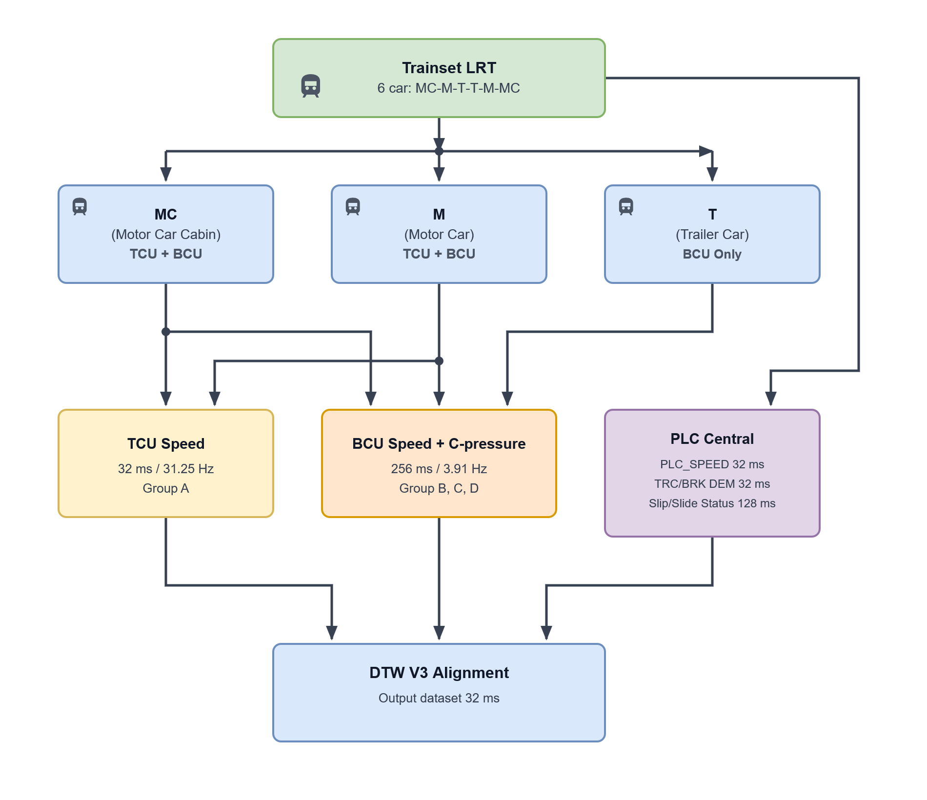
- Hierarchical data source structure of the LRT TCMS dataset
- TCMS Operational Variables in the Pipeline
Variable/Signal | Rate | Proposed |
TCU_MC1_B1_Speed | 32 ms | Motor-car wheel speed;
channel K₁ input |
TCU_M1_B1_Speed | 32 ms | Motor-car (M) wheel speed; channel K₂ input |
BCU_T_B1_Speed_Ax1 | 256 ms | Trailer-axle speed; kinematic reference, channel K₃ |
BCU_MC_Cpressure | 256 ms | Brake-cylinder pressure;
channel K₄ input |
PLC_TRC_BRK_DEM | 32 ms | Traction/braking demand;
channel K₅ input |
PLC_SPEED | 32 ms | Reference trainset speed (absolute) |
PLC_SlipSlide_STS | 128 ms | Conventional WSP status; ground-truth label (0=normal, 1=slip, 2=slide, 3=slip+slide) |
StartDistance | 32 ms | Chainage of the leading bogie; spatial hotspot mapping |
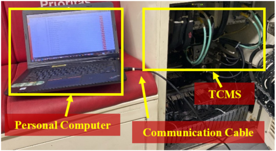
- Data acquisition from the on-board TCMS at the LRT depot
Automated Ground-Truth Labeling
Unlike previous studies that relied on labels annotated by experts, this proposed workflow obtains ground-truth labels directly from the PLC_SlipSlide_STS variable. This variable is identical to the signal used by conventional WSP systems to detect slip-slide events, encoded as a binary status flag updated every 128 ms. Treating it as a label offers three practical advantages: (i) it is generated by certified onboard electronics, not by human operators, thereby eliminating inter-rater inconsistencies; (ii) it scales linearly with the logger’s operational time, so a one-hour log directly yields ~28,000 monitored samples; and (iii) it makes the dataset directly auditable based on the operator’s own incident reports. The labeling procedure follows three steps. First, the raw PLC_SlipSlide_STS stream is upsampled to 32 ms using nearest-neighbor interpolation to synchronize with the master clock. Second, isolated single-sample transitions with durations less than 64 ms are filtered out as electrical noise, since the WSP latch on the LRT communication network physically cannot flip that quickly. Third, each consecutive block with label = 1 is recorded as a single slip event, indexed by its initial time tPLC, which then serves as the reference for the early detection margin. Following this procedure, the 50-minute training log contains 28 distinct slip events and 11,961 individual time-step slip samples, compared to 81,794 normal samples (87.23% vs. 12.77%), confirming the imbalance addressed by class weighting in Section III.E.
Multi-Rate Synchronization via DTW
To enable joint feature extraction across all variables, an upsampling-then-alignment pipeline is implemented (Fig. 3). Continuous variables are upsampled to the finest 32 ms rate using cubic spline interpolation, as implemented in the SciPy library [22]. Binary variables are upsampled via nearest-neighbor interpolation to preserve discrete logic semantics. Following upsampling, fine alignment is performed via DTW, which is well suited to synchronising signals acquired at nonuniform sampling rates [23]. Given two sequences X = (x₁, …, xₙ) and Y = (y₁, …, yₙ) with potential phase misalignment, DTW computes the optimal alignment path π* by minimising the cumulative L₂ distance. The (1) defines the local cost between two points; the (2) defines the dynamic-programming recursion that produces D(i,j) and that returns the optimal alignment path.
subject to the boundary, monotonicity, and continuity constraints standard for DTW. The optimal alignment is then π* = arg min Σ d(i, j) along the path, while the cumulative cost D(m, n) gives the total alignment cost.
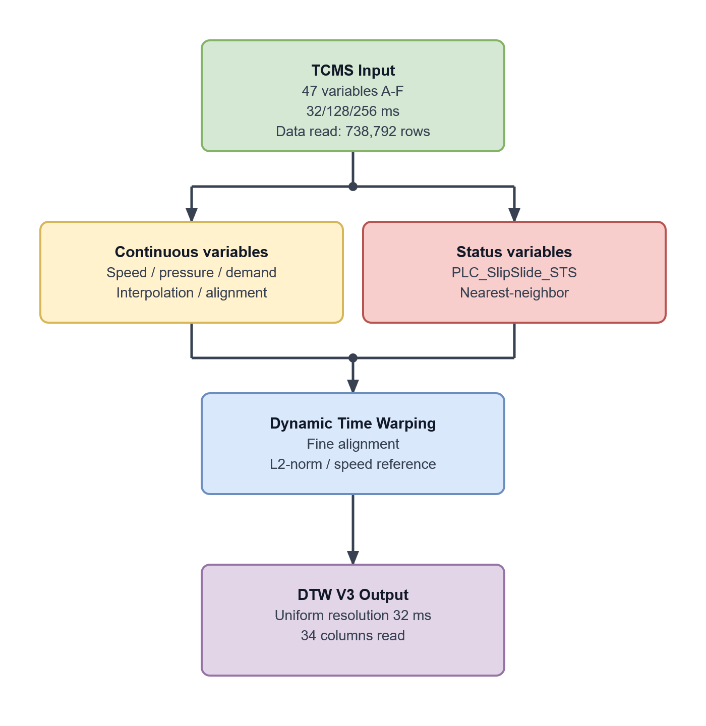
- Multi-rate preprocessing pipeline
Five-Channel Wavelet Feature Extraction
To sharpen the sensitivity to rapid signal transitions, each channel is first transformed into an angular-gradient representation, defined in (3), where k = 8 corresponds to a 0.256 s window at the 32 ms sampling rate. The Continuous Wavelet Transform (CWT) is then applied to this representation. For a signal S(t) with mother wavelet ψ at scale α and time t, the CWT is defined by equation (4), where ψα(t) is the wavelet kernel scaled by α and * denotes convolution [10]. The Morlet wavelet is used here because its Gaussian-modulated oscillatory structure closely matches the morphology of the transient events present in vehicle dynamics, and continuous wavelet transforms of this form effectively extract transient fault features from machinery signals [24].

| (3) |

| (4) |
Five channels are extracted as listed in Table 4. Channel K₃ is the principal methodological contribution. Because the trailer car has no active traction, its BCU-measured speed approximates the true kinematic velocity of the trainset, providing an internal kinematic reference. The differential between the motor-driven TCU speed and the trailer BCU speed therefore directly reveals traction-induced slip. The CWT is computed over scales α ∈ [1, 128] using the PyWavelets library [25], yielding a 128-dimensional feature vector per channel per timestep. Fig. 4 shows representative scalograms of the five channels during a single slip event.
- Five Wavelet Feature Channels
Channel | Input Signal to CWT |

| φ from TCU_MC_B1_SPEED |

| φ from TCU_M_B1_SPEED |

| φ from (TCU_MC-BCU_T) |

| φ from BCU_*_Cpressure |

| φ from PLC_TRC_BRK_DEM |

- Representative wavelet scalograms of the five feature channels during a single slip event
LSTM+MLP Architecture
The proposed architecture follows a multi-stream design (Fig. 5). Each of the five wavelet channels is fed to an independent stacked LSTM with three layers (50, 90 and 60 neurons, respectively) and a dropout of 0.2 between layers. The five LSTM outputs (60 dimensions each) are concatenated with five raw signal values, producing a 305-dimensional vector that is then passed to a two-layer MLP (128 and 64 neurons, ReLU activation [26]) followed by a sigmoid output neuron. The network is trained end-to-end with the Adam optimizer [27], an adaptive first-order method that combines momentum with per-parameter learning-rate scaling and remains a robust default for deep-network training. The full hyperparameter configuration is listed in Table 5.
At each timestep, the LSTM cell evaluates the forget, input, and output gates of (5); these gates regulate how much past information is kept and how much new information is added to the cell state Cₜ, which produces the hidden output hₜ. After the LSTM streams, the dense MLP block computes the pre-activation z and the ReLU activation a of (6); the sigmoid layer at the end of the MLP returns the slip probability ŷ, which is thresholded by T to produce the binary slip / normal decision C̃.
The class weighting {0:1, 1:6.83} compensates for the 6.83: 1 imbalance in the training set, following the rare-events methodology of King and Zeng [28]. The early-detection margin is defined in (7), where  is the first time the conventional WSP fires and
  is the first time the model output exceeds the classification threshold. A positive indicates early detection.

| (7) |

- Proposed multi-stream LSTM+MLP architecture. Five parallel LSTM branches process the five CWT channels independently before concatenation and joint MLP classification
- Hyperparameter Configuration
Parameter | Value |
LSTM Streams | 5 (one per channel) |
LSTM layers per stream | 3 |
Neurons per LSTM layer | 50, 90, 60 |
MLP hidden units | 128, 64 |
Dropout rate | 0.2 |
Optimizer | Adam (lr = 0.0008) |
Batch Size | 32 |
Windows length | 62 timesteps (2 s) |
Class weight | 6.83 |
Max Epoch/patience | 250 / 30 |
Classification threshold | 0.158 (PR-optimized) |
Experimental Results
Wavelet Channel Analysis
Statistical separability of each channel is assessed using the Kolmogorov–Smirnov (KS) two-sample test [29], Cohen's d effect size [30], Fisher's discriminant ratio, and the area under the ROC curve (AUC). The term "discrimination analysis" here refers to the standard practice of measuring, before training a classifier, how well each candidate feature already separates the two classes. If a feature cannot separate the classes in distribution, no classifier will recover the information later. Table 6 presents the discrimination dashboard for the five wavelet channels.
The motor–trailer differential channel (K₃) achieves the highest KS statistic (0.864) and Cohen's d of 1.615, exceeding the "large effect" threshold of 0.8 [31]. Channel K₅ exhibits negligible standalone discrimination (d = −0.050), suggesting that control inputs alone cannot distinguish slip without coupling with kinematic responses. Channels K₁ and K₂ achieve moderate effect sizes (Cohen's d ≈ 0.7), confirming the value of axle-level dynamics. These results validate the methodological choice to exploit the MC–M–T structural hierarchy as a feature engineering principle.
- Wavelet Channel Discrimination Analysis
Ch. | KS | KS p | Cohen d | Fisher | AUC |
K₁ | 0.450 | <0.001 | 0.697 | 0.376 | 0.594 |
K₂ | 0.500 | <0.001 | 0.746 | 0.445 | 0.586 |
K₃ | 0.864 | <0.001 | 1.615 | 2.094 | 0.608 |
K₄ | 0.742 | <0.001 | 1.688 | 1.699 | 0.501 |
K₅ | 0.299 | <0.001 | −0.050 | 0.002 | 0.583 |
Model Classification Performance
The model was trained for up to 250 epochs with early stopping on validation F1-score (patience 30). Test-set evaluation produced the confusion matrix shown in Fig. 6, with the corresponding classification metrics listed in
Table 7.
The proposed model achieves F1 = 0.9272 and AUC = 0.9958, substantially exceeding the wavelet-only threshold baseline (F1 = 0) and the Random Forest baseline (F1 = 0.696). The improvement over the threshold baseline confirms the value of the wavelet feature representation, while the improvement over Random Forest demonstrates the necessity of sequential temporal modeling [18].
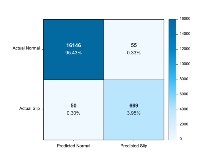
- Confusion matrix of the proposed LSTM+MLP model on the test set. The model correctly classifies 16,146 normal observations and 669 slip observations, with only 55 false positives and 50 false negatives
- Test-Set Performance Comparison
Model | Prec. | Rec. | F1 | AUC |
Wavelet + Threshold | 0.000 | 0.000 | 0.000 | 0.496 |
Decision Tree (wavelet) | 0.571 | 0.426 | 0.488 | 0.706 |
Random Forest (wavelet) | 0.703 | 0.690 | 0.696 | 0.982 |
Proposed (LSTM+MLP) | 0.924 | 0.931 | 0.927 | 0.996 |
Early Detection Capability
For each of the six slip events in the test set, the early detection margin Δt defined in (7) is computed. Table 8 summarizes the per-event results, and Table 9 lists the aggregate statistics. Fig. 7 visualises the distribution of these margins across the six events.
- Early Detection on The Test Set
Event | (s) | (s) | 
| Detected |
1 | 165.760 | 164.864 | 0.896 | Yes |
2 | 984.800 | 983.840 | 0.960 | Yes |
3 | 985.184 | 983.840 | 1.344 | Yes |
4 | 1333.890 | 1329.634 | 4.256 | Yes |
5 | 2125.919 | 2125.087 | 0.832 | Yes |
6 | 2132.287 | 2125.087 | 7.200 | Yes |
- Wavelet Aggregate Early Detection Statistics
Statistic | Value (s) |
Mean Δt | 2.581 |
Median Δt | 1.152 |
Standard deviation | 2.615 |
Q1 (25th percentile) | 0.912 |
Q3 (75th percentile) | 3.528 |
Min Δt | 0.832 |
Max Δt | 7.200 |
% events with Δt > 0 | 100.0% |

- Distribution of early-detection margin Δt across the six test-set slip events. The median margin of 1.152 s with 100% of events satisfying Δt > 0 confirms consistent early detection ahead of the conventional WSP system
The median Δt of 1.152 s, with 100% of events detected ahead of the conventional WSP system, demonstrates consistent early-detection capability. This temporal margin enables preemptive interventions: gradual brake pressure modulation, sand injection activation, or Automatic Train Operation (ATO) speed profile adjustment in pre-mapped slip-prone zones [32].
Spatial Mapping of Slip Hotspots
A complementary spatial analysis is performed on an extended dataset of 5,948 slip-slide events collected from multiple logger sessions covering six trainsets and three operational lines (Line 1; Line 2; Line 3). Each event is geo-localized by converting the native TCMS StartDistance variable to chainage KM, then aggregated into 50-m zones. A composite priority score,

| (8) |
classifies each zone as HIGH (P ≥ 10), MEDIUM (5 ≤ P < 10), or LOW (P < 5), where = 2 for combined gradient–curve, 1 for gradient or curve only, and 0 for straight flat track.
Fig. 8 maps the resulting slip-hotspot density across the three operational lines, with colour encoding the risk level and bar thickness the zone priority score. The aggregation yields 897 unique zones with the following risk distribution: 414 HIGH (46.2%), 290 MEDIUM (32.3%), and 193 LOW (21.5%). Of the events, 68.2% occur on combined gradient–curve geometry, 27.2% on gradient-only segments, and 4.6% on straight track, confirming the dominant role of geometric interaction in slip causation [4], [33]. The top-priority zone (KM −2+350 to −2+300 on Line 2) achieves a priority score of 312.97, more than 2.5 times the median score of the top twenty list and approximately four times the score of the tenth-ranked zone, indicating an extreme localised hotspot. The five highest zones on Line 2 (priority scores of 312.97, 277.56, 229.46, 198.68, and 193.85) all share GRADIENT + CURVE geometry, providing a clear operational target for grinding, sand-box reinforcement, or WSP threshold modulation.
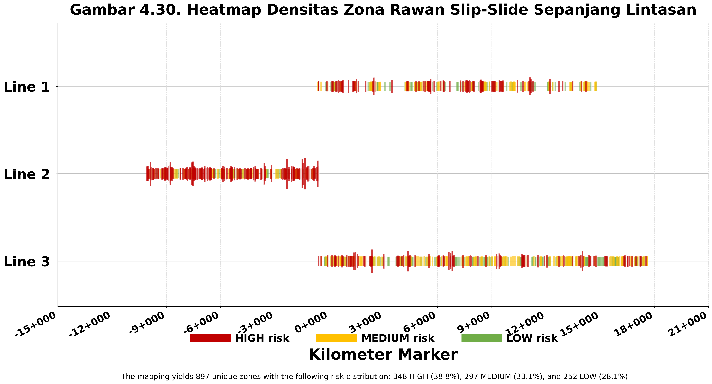
- Spatial slip-hotspot density map across the three operational lines of LRT in Jakarta. Colour encodes the risk level (red = HIGH,
yellow = MEDIUM, green = LOW); bar thickness encodes
the zone priority score
Temporal Distribution of Slip-Slide Events
Beyond the spatial localisation reported in Section IV.D, the timestamp of each event allows a complementary analysis of the daily operational cycle. Events are partitioned into four operational time categories aligned with the LRT timetable structure. Table 10 reports the event-type breakdown per time category. The Morning window is overwhelmingly dominated by pure Slip events (1,896 of 2,124, or 89.3 %), while slide and combined Slip + Slide events together account for only 10.7 % of morning events. By contrast, the Midday, Afternoon and Evening windows show a relatively higher fraction of Slide events (around 15 % of each window), suggesting that the late-morning to evening period exposes the train to slightly different wheel–rail interaction regimes from those experienced at dawn.
Three operational interpretations follow. First, the morning concentration is physically consistent with low-adhesion conditions at dawn: residual moisture, dew formation, and the cooler early-morning rail temperature reduce the available wheel–rail friction, while passenger demand simultaneously imposes the heaviest acceleration cycles on the trainset. Second, the morning category is dominated by pure Slip events (traction-side) rather than Slide events (brake-side), which is consistent with the high-torque acceleration regime characteristic of the morning peak service. Third, the higher Slide fraction observed during Midday, Afternoon, and Evening windows likely reflects a shift toward braking-dominated micro-events as the operational profile transitions from acceleration-heavy morning services to a more balanced service mix later
in the day.
- Event-Type Breakdown by Operational Time Category
Category | Operating Hours | Slip | Slide | Slip +Slide | Total | % of Dataset |
Morning | 05:00-10:00 | 1,896 | 98 | 130 | 2,124 | 35.7% |
Midday | 10:00-14:00 | 908 | 186 | 56 | 1,150 | 19.3% |
Afternoon | 14:00-18:00 | 1,184 | 205 | 82 | 1,471 | 24.7% |
Evening | 18:00-22:00 | 989 | 181 | 33 | 1,203 | 20.2% |
Total |
| 4,977 | 670 | 301 | 5,948 | 100% |
Discussion
Table 11 positions this work relative to prior literature. The F1-score of 0.9272 does not reach the 0.9994 reported by Namoano [9] for adhesion-limited slip on DMU operation. This gap is attributable to (i) dataset volume (50 minutes vs. one year of operation), (ii) operational profile (urban LRT with frequent braking vs. inter-city diesel), and (iii) annotation strategy (automated PLC labels vs. expert-curated annotations). The first two factors are contextual rather than methodological, while the third is arguably an advantage in scalability and reproducibility. Our median early-detection margin of 1.152 s is of the same operational order as the 2.5 s prediction horizon reported by Xiong et al. [19] for a signaling-integrated CNN–GRU predictor, although the two are obtained on different rolling stock and label conventions and are therefore not directly comparable.
- Comparison with Slip Detection Methods
Method | Train Type | Dataset | F1 |
Namoano (2022) [8] | Diesel DMU | 12M obs. | 0.980 |
Namoano (2024)-TL [9] | Diesel DMU | 160K seg. | 0.993 |
Xiong (2026) [19] | EMU (Metro) | TCMS signals | 0.868 |
Proposed | LRT (urban) | 93K timestep | 0.927 |
The median early-detection margin of 1.152 s enables three practical applications: (i) adaptive WSP threshold modulation based on real-time risk assessment; (ii) targeted sand-box deployment at identified hotspots, consistent with Wang [32] reporting that lower WSP thresholds reduce wheel-tread wear by up to 30%; and (iii) predictive maintenance scheduling guided by spatial hotspot data. With 414 HIGH-risk zones identified across the three lines, operators can prioritize inspection and rail-grinding operations on zones with the highest priority scores, potentially reducing maintenance costs by 30% as suggested by Ghiasi [17].
Three limitations warrant discussion. First, the 50-minute dataset for the model training limits broad generalization claims; the 5,948-event spatial dataset is broader but does not reuse the trained model across all sessions. Second, the chainage-based spatial mapping inherits accuracy from the native TCMS StartDistance integration; periodic balise-based reset is required to bound drift. Third, severity-weighted slip mapping that integrates probabilistic outputs from the LSTM model has not yet been explored. Future work will (i) extend the model to multi-corridor LRT systems in Indonesia, (ii) explore attention-based architectures [34] for improved sensitivity to micro-slip events, and (iii) optimize real-time deployment through model quantization [35].
Conclusion
This paper introduced a multi-channel wavelet–LSTM framework for early wheel slip detection in urban LRT, validated on operational TCMS data from LRT in Jakarta. The framework exploits LRT trainset hierarchy through a five-channel CWT feature extraction strategy, with the motor–trailer differential channel achieving Cohen's d = 1.615. The integrated LSTM+MLP achieved F1 = 0.9272 and AUC = 0.9958 on the test set, with a median early-detection margin of 1.152 s preceding conventional WSP activation. A complementary chainage-based spatial mapping derived from a 5,948-event multi-trainset dataset identifies 414 HIGH-risk zones across the three operational lines, providing the first systematic spatial prioritization for an Indonesian LRT corridor. By exploiting the explicit motor–trailer hierarchy of the LRT trainset, the proposed framework extends the wavelet–LSTM paradigm to the urban LRT context and provides a foundation for predictive WSP threshold modulation, sandbox placement, and rail-wear-aware maintenance scheduling. Two directions stand out for future work. First, real-time on-board deployment will be pursued through model quantization and explicit latency budgeting, so that the early-detection margin reported here can be realised within the train control loop. Second, the spatial mapping will be made severity-aware by folding the model's probabilistic slip output into the zone-priority score, turning the present count-based prioritisation into a risk-weighted one.
Acknowledgment
The authors would like to thank the Department of Electrical Engineering at Universitas Sebelas Maret for its academic guidance. This research is funded partially by Sebelas Maret University under the grant of Penelitian Penguatan Kapasitas Grup Riset (PKGR-UNS) A with contract number 371/UN27.22/PT.01.03/2026.
References
- G. J. Krishnan, J. Moraal, Z. Li, and Z. Yang, “An Experimental Study of Wheel–Rail Creep Curves Under Dry Contact Conditions Using V-Track †,” Lubricants, vol. 13, no. 7, 2025, https://doi.org/10.3390/lubricants13070287.
- M. N. Tawfik, M. M. Padzi, S. Abdullah, D. Harmanto, M. N. Firdaws, and H. Hapaz, “A Review of the Rolling Contact Fatigue of Rail Wheels Under Various Stresses,” Journal of Failure Analysis and Prevention, vol. 23, no. 1, pp. 16–29, 2023, https://doi.org/10.1007/s11668-022-01568-6.
- S. Gulcimen, E. K. Aydogan, and N. Uzal, “Life cycle sustainability assessment of a light rail transit system: Integration of environmental, economic, and social impacts,” Integrated Environmental Assessment and Management, vol. 17, no. 5, pp. 1070–1082, 2021, https://doi.org/10.1002/ieam.4428.
- G. Mei and G. Chen, “Slip of wheels on rails: The root cause for rail undulant wear,” Wear, vol. 523, no. 12, p. 204727, 2023, https://doi.org/10.1016/j.wear.2023.204727.
- B. Allotta, L. Pugi, M. Malvezzi, F. Bartolini, and F. Cangioli, “A scaled roller test rig for high-speed vehicles,” Vehicle System Dynamics, vol. 48, no. SUPPL. 1, pp. 3–18, 2010, https://doi.org/10.1080/00423111003663576.
- T. X. Mei, J. H. Yu, and D. A. Wilson, “a mechatronic approach for anti-slip control in railway traction,” in IFAC Proceedings Volumes, pp. 8275–8280, 2008, https://doi.org/10.3182/20080706-5-kr-1001.01399.
- T. F. Zhu et al., “Experimental study on the influence of slip ratio on irregular wear behaviors of wheel/rail,” Wear, vol. 523, no. 1, p. 204780, 2023, https://doi.org/10.1016/j.wear.2023.204780.
- B. Namoano, C. Ruiz-Carcel, C. Emmanouilidis, and A. G. Starr, “Data-Driven Wheel Slip Diagnostics for Improved Railway Operations,” in IFAC-PapersOnLine, pp. 103–108, 2022, https://doi.org/10.1016/j.ifacol.2022.09.191.
- B. Namoano, C. Emmanouilidis, and A. Starr, “Detecting wheel slip from railway operational data through a combined wavelet, long short-term memory and neural network classification method,” Engineering Applications of Artificial Intelligence, vol. 137, no. PB, p. 109173, 2024, https://doi.org/10.1016/j.engappai.2024.109173.
- S. Mallat, “Fourier kingdom,” in A Wavelet Tour of Signal Processing, pp. 20–41, 1999, https://doi.org/10.1016/b978-012466606-1/50004-0.
- A. Orhan, N. Yordanov, M. Ertarğın, M. Zhilevski, and M. Mikhov, “A Comparative Study of Time–Frequency Representations for Bearing and Rotating Fault Diagnosis Using Vision Transformer,” Machines, vol. 13, no. 8, pp. 1–21, 2025, https://doi.org/10.3390/machines13080737.
- Q. Wang, Y. Yu, H. O. A. Ahmed, M. Darwish, and A. K. Nandi, “Open-circuit fault detection and classification of modular multilevel converters in high voltage direct current systems (Mmc-hvdc) with long short-term memory (lstm) method,” Sensors, vol. 21, no. 12, 2021, https://doi.org/10.3390/s21124159.
- H. S. Oh and J. M. Kim, “Data-Driven AI Model for Railway Vehicle SIV Condition Diagnosis System,” Journal of Electrical Engineering and Technology, vol. 20, no. 7, pp. 4725–4737, 2025, https://doi.org/10.1007/s42835-025-02428-7.
- K. Kim, S. H. Kong, and S. Y. Jeon, “Slip and Slide Detection and Adaptive Information Sharing Algorithms for High-Speed Train Navigation Systems,” IEEE Transactions on Intelligent Transportation Systems, vol. 16, no. 6, pp. 3193–3203, 2015, https://doi.org/10.1109/TITS.2015.2437899.
- R. Tang et al., “A literature review of Artificial Intelligence applications in railway systems,” Transportation Research Part C: Emerging Technologies, vol. 140, no. May, p. 103679, 2022, https://doi.org/10.1016/j.trc.2022.103679.
- Z. Jin, J. Shang, Q. Zhu, C. Ling, W. Xie, and B. Qiang, “RFRSF: employee turnover prediction based on random forests and survival analysis,” in Lecture Notes in Computer Science (including subseries Lecture Notes in Artificial Intelligence and Lecture Notes in Bioinformatics), pp. 503–515, 2020, https://doi.org/10.1007/978-3-030-62008-0_35.
- R. Ghiasi, M. A. Khan, D. Sorrentino, C. Diaine, and A. Malekjafarian, “An unsupervised anomaly detection framework for onboard monitoring of railway track geometrical defects using one-class support vector machine,” Engineering Applications of Artificial Intelligence, vol. 133, no. PB, p. 108167, 2024, https://doi.org/10.1016/j.engappai.2024.108167.
- Y. Lecun, Y. Bengio, and G. Hinton, “Deep learning,” Nature, vol. 521, no. 7553, pp. 436–444, 2015, https://doi.org/10.1038/nature14539.
- W. Zha, D. Ou, Y. Tong, C. Xu, S. Su, and J. Xiong, “Train Slide Prediction and Risk Assessment Using Vehicle-Signal Data: A Data-Model Fusion Method,” Urban Rail Transit, 2026, https://doi.org/10.1007/s40864-026-00269-9.
- Y. Chen, X. Liu, W. Fan, N. Duan, and K. Zhou, “A deep-LSTM-based fault detection method for railway vehicle suspensions,” Machines, vol. 12, no. 2, pp. 1–13, 2024, https://doi.org/10.3390/machines12020116.
- A. Lourenço, D. Ribeiro, M. Fernandes, and G. Marreiros, “Time series data mining for railway wheel and track monitoring: a survey,” Neural Computing and Applications, vol. 36, no. 27, pp. 16707–16725, 2024, https://doi.org/10.1007/s00521-024-10138-w.
- P. Virtanen et al., “SciPy 1.0: fundamental algorithms for scientific computing in Python,” Nature Methods, vol. 17, no. 3, pp. 261–272, 2020, https://doi.org/10.1038/s41592-019-0686-2.
- Y. Jiang et al., “EventDTW: An improved dynamic time warping algorithm for aligning biomedical signals of nonuniform sampling frequencies,” Sensors (Switzerland), vol. 20, no. 9, 2020, https://doi.org/10.3390/s20092700.
- J. Du, X. Li, Y. Gao, and L. Gao, “Integrated Gradient-Based Continuous Wavelet Transform for Bearing Fault Diagnosis,” Sensors, vol. 22, no. 22, 2022, https://doi.org/10.3390/s22228760.
- G. Lee, R. Gommers, F. Waselewski, K. Wohlfahrt, and A. O’Leary, “PyWavelets: A Python package for wavelet analysis,” Journal of Open Source Software, vol. 4, no. 36, p. 1237, 2019, https://doi.org/10.21105/joss.01237.
- A. Maniatopoulos and N. Mitianoudis, “Learnable Leaky ReLU (LeLeLU): An Alternative Accuracy-Optimized Activation Function,” Information (Switzerland), vol. 12, no. 12, 2021, https://doi.org/10.3390/info12120513.
- W. Cheng, R. Pu, and B. Wang, “AMC: Adaptive Learning Rate Adjustment Based on Model Complexity,” Mathematics, vol. 13, no. 4, 2025, https://doi.org/10.3390/math13040650.
- G. King and L. Zeng, “Logistic regression in rare events data,” Journal of Statistical Software, vol. 8, pp. 137–163, 2003, https://doi.org/10.18637/jss.v008.i02.
- D. T. Nguyen, T. K. Nguyen, Z. Ahmad, and J. M. Kim, “A Reliable Pipeline Leak Detection Method Using Acoustic Emission with Time Difference of Arrival and Kolmogorov–Smirnov Test,” Sensors, vol. 23, no. 23, 2023, https://doi.org/10.3390/s23239296.
- A. Pérez-Torres, J. Navarrete-Campos, R. V. Sánchez, and S. Barceló-Cerdá, “Selection of Vibration Signal Features in the Frequency Domain to Determine the Level of Failure Severity in Spur Gearboxes,” Journal of Vibration Engineering and Technologies, vol. 13, no. 8, 2025, https://doi.org/10.1007/s42417-025-02213-w.
- T. Saito and M. Rehmsmeier, “The precision-recall plot is more informative than the ROC plot when evaluating binary classifiers on imbalanced datasets,” PLoS ONE, vol. 10, no. 3, pp. 1–21, 2015, https://doi.org/10.1371/journal.pone.0118432.
- R. Wang, Y. Yang, P. Liu, and P. Allen, “A comparative study of WSP control methods: Effects on wear and RCF evolution in railway wheels,” Wear, vol. 572–573, no. February, p. 206049, 2025, https://doi.org/10.1016/j.wear.2025.206049.
- O. Polach, “Creep forces in simulations of traction vehicles running on adhesion limit,” Wear, vol. 258, no. 7–8, pp. 992–1000, 2005, https://doi.org/10.1016/j.wear.2004.03.046.
- K. Mohiuddin et al., “Retention Is All You Need,” in International Conference on Information and Knowledge Management, Proceedings, pp. 4752–4758, 2023, https://doi.org/10.1145/3583780.3615497.
- S. Han, H. Mao, and W. J. Dally, “Deep compression: Compressing deep neural networks with pruning, trained quantization and Huffman coding,” 4th International Conference on Learning Representations, ICLR 2016 - Conference Track Proceedings, 2016, http://arxiv.org/abs/1510.00149
Yulian Lingga Permana, A Multi-Channel Wavelet Long Short-Term Memory Framework for Early Wheel Slip Detection in Urban Light Rail Transit





