Comparative Analysis of Random Forest and LSTM for Predictive Maintenance of Electric Motors

Muhammad ‘Atiq 1,*, Musab Ali El Nefati 2, Arief Marwanto 3, Fajar Husain Asy'ari 4, Rio Subandi 5, Danang Hendrawan 6,

1, 6 Department of Electrical Engineering, Sekolah Tinggi Teknik Pati, Pati, Indonesia

2 Department of Computer Engineering, High Institute of Industrial Technology-Engila, Libya

3 Department of Electrical Engineering, Universitas Islam Sultan Agung Semarang, Semarang, Indonesia

4, 5 Department of Informatics Engineering, Sekolah Tinggi Teknik Pati, Pati, Indonesia

Email: 1 atiq.corps@gmail.com, 2 mosabalnfatti@gmail.com, 3 arief@unissula.ac.id, 4 fajarhusain@sttp.ac.id,
5 riosubandi9@gmail.com, 6 dananghendrawan70@gmail.com

*Corresponding Author

Abstract—This study presents a comparative analysis of Random Forest and Long Short-Term Memory (LSTM) algorithms for predictive maintenance of electric motors using Industrial Internet of Things (IIoT) sensor data (current, temperature, vibration). A synthetic dataset from Kaggle comprising 5,000 samples across three operational states (HEALTHY, WARNING, CRITICAL) was employed. Experiments were conducted on Google Colab with a Tesla T4 GPU. The LSTM model achieved a classification accuracy of 98.9%, outperforming Random Forest (98.5%), with perfect precision and recall for the WARNING state and improved recall for the CRITICAL state (0.97 vs. 0.96). However, Random Forest demonstrated substantially shorter training time (2 seconds vs. 30 seconds). For real-time industrial deployment on Programmable Logic Controllers (PLCs), Random Forest is recommended due to its rapid inference (5-10 ms), while LSTM is better suited for critical assets where detection accuracy is prioritized. The findings also confirm the viability of Google Colab as an accessible platform for predictive maintenance research in academic settings. This work contributes a practical framework for selecting between machine learning and deep learning approaches in IIoT-based motor fault diagnosis.

Keywords—Predictive Maintenance; Random Forest; Electric Motor; Industrial Internet of Things

1. Introduction

The widespread implementation has revolutionized contemporary manufacturing through real-time monitoring capabilities and data-informed decision-making processes. Networks and Random Forest Algorithms [1]. Among the most essential IIoT applications is predictive maintenance, which facilitates the early identification of equipment malfunctions prior to their occurrence, consequently minimizing unplanned downtime, reducing repair expenses, and prolonging operational lifespan [2].

Conventional industrial environments typically employ either reactive or scheduled maintenance approaches. Reactive maintenance intervenes solely after failures manifest, leading to expensive production interruptions [3]. Preventive maintenance, though relatively superior, adheres to predetermined timetables irrespective of actual equipment conditions, generating superfluous servicing activities and possible over-maintenance [4]. Predictive maintenance surmounts these constraints by persistently observing equipment condition via sensor inputs and initiating maintenance solely upon identification of deterioration trends.

Electric motors constitute vital elements within industrial apparatus, propelling conveyors, pumps, fans, and compressors. Motor malfunctions can cause considerable production deficits and safety threats [5]. Frequent failure categories encompass bearing degradation, stator winding defects, rotor imbalance, and thermal excess [6]. These failures typically appear through quantifiable variations in operational indicators like current draw, thermal levels, and vibration frequency, rendering them identifiable using machine learning approaches [7].

Recent progress in machine learning has facilitated the creation of predictive maintenance frameworks employing sensor data. Random Forest, an ensemble learning method, has gained extensive acceptance due to its resilience, capacity to manage non-linear correlations, and defense against overfitting [8]. Nevertheless, Random Forest processes each data point separately without explicitly capturing temporal relationships, potentially constraining its efficacy for recognizing progressive deterioration sequences [9].

Deep learning methodologies, notably Long Short-Term Memory (LSTM) architectures, have become compelling substitutes for time-series prediction challenges. LSTM is purposefully engineered to retain long-range dependencies within sequential information, rendering it appropriate for representing degradation pathways that develop gradually [10]. Numerous investigations have validated LSTM's efficacy for remaining useful life (RUL) prediction and anomaly identification within industrial machinery [11].

Notwithstanding these developments, a deficiency persists in comparative investigations assessing both conventional machine learning (Random Forest) and deep learning (LSTM) for multi-category predictive maintenance employing IIoT sensor data. Moreover, restricted research has examined the deployment of such frameworks utilizing accessible cloud computing infrastructures like Google Colab, which could broaden predictive maintenance instruction and investigation within resource-limited academic environments.

The central problem addressed in this study is the lack of a systematic comparative framework for selecting between Random Forest and LSTM algorithms in the context of multi-class predictive maintenance for electric motors.

While both methods have been individually applied to fault detection tasks, the literature offers limited guidance on their relative strengths and weaknesses when confronted with the specific challenges of IIoT data: high dimensionality, temporal dependencies, and imbalanced class distributions (HEALTHY, WARNING, CRITICAL). This gap is particularly critical for industrial practitioners who require not only high accuracy but also interpretability, computational efficiency, and real-time deployability on resource-constrained platforms such as Programmable Logic Controllers (PLCs). By providing a direct head-to-head comparison under controlled conditions, this study aims to offer a practical decision framework that explicitly accounts for the trade-offs between prediction accuracy, training speed, and inference latency, thereby moving beyond generic descriptions to actionable engineering insights.

This study extends the existing literature in three significant ways. First, unlike previous comparative works in business analytics [12] or solar energy forecasting [13], which focused on regression tasks, our research specifically targets a three-class classification problem (HEALTHY, WARNING, CRITICAL) that mirrors the actual operational states of industrial motors. Second, we provide a systematic evaluation of both models using a synthetic dataset that includes controlled degradation patterns, enabling a clearer assessment of each algorithm's sensitivity to temporal dynamics and class imbalance. Third, and most importantly, we explicitly analyze the deployment pathways of both models on industrial PLCs—a practical consideration often overlooked in academic studies—by examining model conversion to ONNX (for Random Forest) and TensorFlow Lite (for LSTM) formats. This integration of algorithmic performance with hardware constraints distinguishes our work from prior theoretical comparisons and offers tangible value to engineering practitioners.

In comparison to other state-of-the-art techniques, such as Convolutional Neural Networks (CNNs) or hybrid CNN-LSTM models that have been proposed for fault diagnosis [10], our approach deliberately prioritizes simplicity and interpretability without sacrificing performance. Random Forest offers inherent transparency through feature importance ranking, while LSTM provides a principled mechanism for modeling temporal dependencies through its gated architecture. Although our focus is on comparative performance rather than control-theoretic guarantees, we address stability considerations by evaluating model robustness under varying data conditions and discussing potential failure modes (e.g., sensor drift, abrupt faults) in the Discussion section. The reproducibility of our experiments is ensured through the use of Google Colab, which provides a standardized computational environment, and the open publication of our methodology, enabling other researchers to replicate and challenge our findings.

Recent comparative studies in other domains such as solar power forecasting [12], have demonstrated that LSTM generally outperforms Random Forest for time-series prediction tasks. However, these studies did not specifically address multi-class predictive maintenance for electric motors using IIoT sensor data, nor did they explore deployment pathways to industrial PLCs.

This research intends to fill these voids [13] by contrasting Random Forest and LSTM efficacy for early electric motor failure identification using a publicly accessible synthetic motor malfunction dataset. The particular aims include: (i) creating and training both models using sensor data (current, temperature, vibration), (ii) evaluating and comparing their effectiveness via accuracy, precision, recall, F1-score, and confusion matrices, and (iii) appraising their computational efficiency within a Google Colab setting.

2. Materials and Methods

This part details the methodical procedures executed in this study, covering data origin, preprocessing, model design, and performance assessment.

1. Research Flowchart

Fig. 1 illustrates the complete research methodology sequence, depicting the full workflow starting from data procurement to final conclusions.

The research methodology consisted of five main stages: (i) Data acquisition and preprocessing (Kaggle dataset, time step addition, label encoding, Min-Max normalization), (ii) Data splitting (80% training, 20% testing), (iii) Model development (Random Forest as baseline, LSTM with 10-time-step sequences), (iv) Model evaluation (accuracy, precision, recall, F1-score, confusion matrix), and (v) Performance comparison between Random Forest and LSTM

1. Research Methodology Flowchart

1. Dataset Description

The dataset employed in this investigation was sourced from the Kaggle repository under the designation "Synthetic Motor Failure Dataset." This collection simulates sensor measurements from an industrial electric motor operating across three conditions: HEALTHY, WARNING, and CRITICAL.

The complete dataset comprises 5000 samples distributed as follows: 3,000 HEALTHY cases, 1,500 WARNING cases, and 500 CRITICAL cases.

Every sample encompasses four characteristics: Timestamp (recording time indicator), Motor_Current_A (motor current in Amperes), Motor_Temp_C (motor temperature in Celsius), Vibration_Hz (motor vibration frequency in Hertz), and Status (operational category label: HEALTHY, WARNING, CRITICAL).

This dataset was chosen because it satisfies the subsequent research standards: (i) includes three status categories representing the machinery lifecycle, (ii) features time-series information illustrating progressive deterioration patterns, (iii) lacks missing entries, and (iv) possesses adequate data magnitude (5000 samples) for machine learning model training.

2. Data Preprocessing

Prior to model training, the information underwent multiple preprocessing procedures. Initially, missing entries were examined utilizing the isnull() function from the Pandas library. The examination revealed zero missing values across any attribute, eliminating the need for imputation or data removal.

Subsequently, because the dataset lacked an explicit temporal column, a Time_Step column was incorporated to indicate the chronological order in minutes. This column was generated employing the pd.date_range() function with one-minute gaps, producing a total span of 5,000 minutes (approximately 3.47 days).

Third, the operational categories, originally in textual format (HEALTHY, WARNING, CRITICAL), were transformed into numeric equivalents utilizing LabelEncoder from the scikit-learn package. The conversion mapped HEALTHY → 0, WARNING → 1, and CRITICAL → 2. This transformation is essential because machine learning algorithms exclusively handle numeric data.

Fourth, the three sensor characteristics (Motor_Current_A, Motor_Temp_C, Vibration_Hz) exhibit disparate ranges. Current spans 2-6 A, temperature spans 40-130°C, and vibration spans 0-40 Hz. To guarantee equal feature contribution to model computations, data normalization was executed using Min-Max scaling, linearly transforming each feature to the [0,1] interval. The employed formula is:

Min-Max normalization has been broadly embraced in predictive maintenance implementations for IIoT systems [14], [15].

3. Data Splitting

The preprocessed dataset was partitioned into two segments: training set and test set, following an 80:20 proportion. The division was performed using the train_test_split function from scikit-learn with the stratify=y parameter to preserve class distribution proportions across both subsets. The random_state=42 parameter ensured result reproducibility. The data splitting produced 4000 samples for training and 1000 samples for testing [16].

4. Random Forest Model Configuration

Random Forest constitutes an ensemble learning method integrating multiple decision trees to generate more precise and stable predictions [8], [17]. In this investigation, Random Forest served as a baseline model for comparison against LSTM.

The Random Forest model employed n_estimators = 100 (decision tree count) and random_state = 42 (reproducibility). All remaining parameters utilized scikit-learn default settings.

The training procedure involved: (i) feeding training data (4000 samples with 3 features) into the model, (ii) constructing 100 independent decision trees, (iii) training each tree on distinct data subsets (bootstrap sampling), and (iv) determining final predictions through majority voting across all trees. Training duration was quantified using the Python time library.

The prediction mechanism of Random Forest can be formalized as follows. Given a training dataset:

with N samples and M features, the algorithm constructs T decision trees using bootstrap samples.

For each tree t, a random subset of m features (m≪M) is selected at each node to determine the optimal split. The prediction for a new input x is obtained by averaging the predictions from all trees:

where  is the prediction from the t-th decision tree. This ensemble averaging reduces overfitting and improves generalization performance, making Random Forest particularly suitable for high-dimensional datasets with complex feature interactions [18].

5. LSTM Model Configuration

Long Short-Term Memory (LSTM) represents a Recurrent Neural Network (RNN) variant specifically engineered for sequential data handling (time series) [10]. LSTM can retain information from preceding time steps while discarding irrelevant data, rendering it appropriate for identifying progressive deterioration patterns in machinery.

Sequence Generation: Prior to LSTM input, time-series data required conversion into sequences. This study selected sequence length (SEQ_LEN) = 10, meaning the model examines 10 prior data points to forecast the 11th point. From 5000 original samples, 4990 sequences were produced.

Each sequence measured 10 × 3 (10 time steps × 3 features), with labels representing the status at the 11th time step.

Network Structure: The LSTM architecture comprised an input layer accepting sequences sized (10, 3), an initial LSTM layer with 64 units and return_sequences=True, a Dropout layer with 0.2 rate preventing overfitting, a second LSTM layer with 32 units, and an output Dense layer with 3 neurons employing softmax activation to generate class probabilities.

Compilation and Training: The LSTM model was compiled using sparse_categorical_crossentropy loss (appropriate for integer labels 0, 1, 2), the adam optimizer, and accuracy as an evaluation metric. Training proceeded for 30 epochs with a batch size of 32. Training data was further subdivided into 80% training and 20% validation using validation_split=0.2. Class weights addressed data imbalance (more HEALTHY samples than CRITICAL samples).

The LSTM architecture is governed by a set of gating mechanisms that regulate information flow through the network. At each time step t, the LSTM cell updates its internal state using the following equations:

Forget Gate:

Input Gate:

Candidate Cell State:

Cell State Update:

Output Gate:

Hidden State:

where  are the forget, input, and output gate activations;  are the cell state and hidden state;  is the input; are the weight matrices and bias vectors;  is the sigmoid function; and  denotes element-wise multiplication.

These gating mechanisms enable the LSTM to selectively retain or discard information over long sequences, making it well-suited for capturing temporal dependencies in time-series data [19].

6. Computing Environment

All experiments utilized Google Colaboratory (Google Colab) featuring: Tesla T4 GPU (16 GB VRAM), 12 GB RAM, 78 GB storage, Python 3.12 runtime, and primary libraries including TensorFlow 2.x, scikit-learn 1.x, Pandas, NumPy, Matplotlib, and Seaborn. Google Colab was selected due to its free accessibility, reproducibility assurance, and GPU provision, accelerating LSTM model training [20], [21].

7. Evaluation Indicators

Both models were assessed using accuracy, precision, recall, and F1-score. Accuracy represents correct prediction proportion across all samples: (TP + TN) / (TP + TN + FP + FN). Precision indicates the correct positive prediction proportion: TP / (TP + FP). Recall denotes actual positive samples correctly identified: TP / (TP + FN). F1-Score constitutes the harmonic mean of precision and recall: 2 × (Precision × Recall) / (Precision + Recall). Furthermore, confusion matrices were provided, displaying detailed per-class classification outcomes, and training duration was recorded to contrast computational efficiency.

3. Results Findings and Discussion

1. Results

This section presents the experimental outcomes obtained from applying Random Forest and LSTM algorithms for electric motor predictive maintenance. The complete dataset contained 5000 samples categorized as HEALTHY (3000), WARNING (1500), and CRITICAL (500). Model training and inference utilized Google Colaboratory's Tesla T4 GPU to ensure research reproducibility.

2. Exploratory Data Analysis

Table 1 provides descriptive statistics for the three sensor parameters (Motor Current, Motor Temperature, and Vibration) across the three operational conditions.

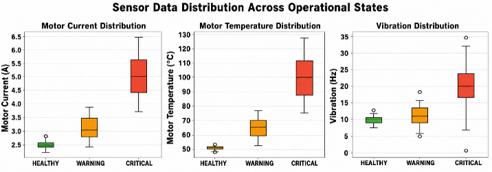
The statistical analysis confirms a distinct progressive degradation pattern. Mean motor current rose from 2.50 A (HEALTHY) to 3.12 A (WARNING) and further to 5.00 A (CRITICAL). Likewise, average temperature increased from 49.5°C to 98.9°C, while mean vibration frequency elevated from 10.0 Hz to 20.4 Hz.

Fig. 2 depicts the temporal progression of all three sensor signals across the 5000-minute observation period. The vertical dashed lines at time steps 3000 and 4500 mark the initiation of WARNING and CRITICAL phases, respectively.

The distribution of each sensor parameter, categorized by operational status, is presented in Fig. 3 using boxplot visualization. Fig. 4 displays the correlation matrix examining relationships between sensor features and the status code. Particularly noteworthy are the strong positive correlations between Motor Current and Motor Temperature (0.90) and between Motor Current and Vibration (0.90).

1. Descriptive Statistics of Sensor Data Across Operational States

2. Sensor Degradation Pattern from Healthy to Critical

3. Sensor Data Distribution Across Operational States

4. Feature Correlation Matrix

1. Random Forest Performance

The Random Forest classifier utilized 80% of the data (4000 samples) for training and the remaining 20% (1000 samples) for testing, employing default hyperparameters (n_estimators=100, random_state=42). Table 2 summarizes the Random Forest classification performance.

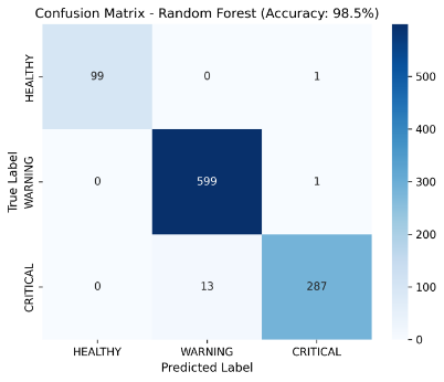
The Random Forest model attained an overall accuracy of 98.5%. While it successfully identified WARNING status (recall = 1.00, precision = 0.98) and HEALTHY status (precision = 1.00), performance for CRITICAL detection was slightly diminished (recall = 0.96), indicating that 4% of actual failures were misclassified. The confusion matrix for Random Forest predictions is presented in Fig. 5.

2. Random Forest Classification Report

5. Confusion Matrix - Random Forest

1. LSTM Performance

The LSTM architecture employed a sequence length of 10 time steps to capture temporal dependencies. The design comprised two LSTM layers (64 and 32 units) with a dropout rate of 0.2 for regularization, concluding with a dense output layer utilizing softmax activation for three-class classification. Table 3 presents the LSTM classification results.

The LSTM model achieved superior accuracy (98.9%), surpassing Random Forest by 0.4%. Notably, it delivered perfect precision across all three categories and flawless recall for the WARNING status. Critical status recall improved to 0.97 compared to 0.96 for Random Forest.

Fig. 6 displays the confusion matrix for the LSTM model. Training progression curves over 30 epochs for the LSTM model are shown in Fig. 7.

3. LSTM Classification Report

(a)

(b)

6. Confusion Matrix – LSTM (a) Confusion Matrix and
   (b) Training Curves

7. LSTM Training Curves

1. Model Comparison

Table 4 offers a direct performance comparison between the two models. In summary, although LSTM achieved marginally higher accuracy (98.9%), Random Forest exhibited substantially faster training speed (2 seconds vs. 30 seconds), rendering it appropriate for real-time deployments with constrained computational resources.

4. Performance Comparison Between Random Forest and LSTM

2. Discussion

The experimental results confirm that both Random Forest and LSTM can effectively classify electric motor status (HEALTHY, WARNING, CRITICAL) with high accuracy (98.5% and 98.9%, respectively). This finding supports the sufficiency of current, temperature, and vibration measurements for dependable predictive maintenance [22].

3. Model Performance Comparison

The demonstrated superiority of LSTM over Random Forest originates from its inherent capacity to model temporal dependencies, which is essential for identifying gradual deterioration from WARNING to CRITICAL states [10]. The perfect precision and recall for the WARNING status achieved by LSTM highlights its reliability for early warning systems.

This aligns with previous comparative research confirming LSTM's advantage for time-series fault diagnosis [23]. The observed 0.4% performance gap between LSTM and Random Forest is narrower than some literature reports, presumably due to the controlled, noise-free characteristics of the synthetic dataset [24].

4. Trade-offs and Industrial Implementation

The practical trade-off between accuracy and computational efficiency is clearly illustrated: LSTM offers higher accuracy but requires 15× longer training time [9]. For real-time control applications on Programmable Logic Controllers (PLCs), such as the Siemens S7-1500, Random Forest is preferred because of its minimal computational footprint and rapid inference (5-10 ms), which meets deterministic scan cycle requirements [25]. In contrast, for critical infrastructure, where maximizing detection accuracy is paramount, LSTM remains the superior choice [26].

Importantly, both models can be deployed on industrial PLCs through conversion to ONNX (for Random Forest) or TensorFlow Lite (for LSTM) formats, enabling edge-based inference without cloud dependency and providing benefits in latency, bandwidth, and data security [7].

5. Implications and Limitations

The successful use of Google Colab's free tier demonstrates that rigorous predictive maintenance research can be conducted without expensive computing infrastructure, increasing educational accessibility [27]. Students can replicate the complete workflow using only a web browser, effectively connecting classroom theory with industrial practice [21].

However, this study has several constraints.

• First, the dataset is synthetic; real-world industrial data typically contains noise and missing values that could degrade model performance [28].
• Second, conclusions are drawn from a single motor type; applicability to other equipment requires additional validation.
• Third, the LSTM architecture was relatively shallow; deeper networks might yield better accuracy at increased computational expense.

The observed superiority of LSTM over Random Forest in this study can be attributed to its ability to model long-term dependencies through its gating mechanisms (forget, input, and output gates). Unlike Random Forest, which treats each data point independently, LSTM retains information across time steps, enabling it to capture the gradual degradation patterns from WARNING to CRITICAL states. However, this advantage is contingent on the availability of sufficient training data; with limited data, LSTM may overfit due to its large number of parameters. Conversely, Random Forest demonstrated robust performance even with fewer training samples, making it a more reliable choice for small datasets or applications with limited historical data.

The proposed models exhibit limitations under certain conditions. First, both models assume that the sensor data are representative of the motor's actual operating conditions. In the presence of sensor drift, missing values, or high-frequency noise, model performance may degrade significantly. Second, the models were trained and validated on a synthetic dataset; their generalizability to real-world industrial data, which often contains outliers and non-stationary patterns, requires further empirical validation. Third, the LSTM model may fail to accurately predict CRITICAL states if the degradation process is abrupt rather than gradual, as the model relies on learning progressive patterns. Under such conditions, Random Forest—which does not depend on temporal ordering—may offer more stable predictions. These boundary conditions highlight the importance of data quality and preprocessing in ensuring reliable predictive maintenance outcomes.

Future research should validate this approach on authentic industrial datasets and investigate deployment on edge-capable PLCs [29].

4. Conclusion

This study compared Random Forest and LSTM for predictive maintenance of electric motors using IIoT sensor data (current, temperature, vibration) derived from a synthetic Kaggle dataset containing 5,000 samples across three operational classes (HEALTHY, WARNING, CRITICAL). LSTM achieved 98.9% accuracy, surpassing Random Forest (98.5%), and delivered perfect precision and recall for the WARNING class while improving recall for CRITICAL failures (0.97 vs. 0.96). However, Random Forest trained significantly faster (2 seconds vs. 30 seconds on a Tesla T4 GPU). For real-time industrial deployment on PLCs (e.g., Siemens S7-1500), Random Forest is recommended due to its lightweight design and fast inference (5-10 ms), which aligns with deterministic PLC scan cycles. Conversely, for critical assets where maximum accuracy is prioritized, LSTM is preferable. Both models can be deployed on edge-enabled PLCs by exporting to ONNX or TensorFlow Lite formats, enabling local inference without cloud dependency. All experiments utilized Google Colab's free tier, highlighting the accessibility of this research for academic institutions. Future work should validate the approach on real-world industrial datasets and implement the models on industrial PLCs.

References

1. A. S. Allahloh, M. Sarfraz, D. Y. Mohammed, N. K. Ibrahim, and H. H. Thary, “From Industrial Automation to Intelligent Automation: The Impact of IIoT on Process Control - A Review,” Iraqi Journal for Computer Science and Mathematics, vol. 6, no. 3, pp. 134–159, 2025, https://doi.org/10.52866/2788-7421.1281.
2. R. Kumar, M. Mishra, S. Suman, and P. Singh Bali, “Predictive Maintenance in Industrial Systems Using Machine Learning,” International Journal of Innovative Science and Research Technology (IJISRT), vol. 15, no. 4, pp. 1778–1785, 2024, https://doi.org/10.38124/ijisrt/ijisrt24mar1367.
3. A. Enemosah and O. G. Ifeanyi, “SCADA in the Era of IoT: Automation, Cloud-driven security, and machine learning applications,” International Journal of Science and Research Archive, vol. 13, no. 1, pp. 3417–3435, 2024, https://doi.org/10.30574/ijsra.2024.13.1.1975.
4. A. Nechibvute and H. D. Mafukidze, “Integration of SCADA and Industrial IoT: Opportunities and Challenges,” IETE Technical Review (Institution of Electronics and Telecommunication Engineers, India), vol. 41, no. 3, pp. 312–325, 2024, https://doi.org/10.1080/02564602.2023.2246426.
5. H. El hadraoui, A. El maghraoui, O. Laayati, E. Sabani, M. Zegrari, and A. Chebak, “AI-driven diagnosis and health management of autonomous electric vehicle powertrains: An empirical data-driven approach,” Results in Engineering, vol. 27, p. 106157, 2025, https://doi.org/10.1016/j.rineng.2025.106157.

6. M. Michel, A. Mehanna, S. N. Saleh, and A. S. Shehata, “Proactive fault prediction in marine diesel engines using multivariate machine learning,” Scientific reports, vol. 16, no. 1, p. 9678, 2026, https://doi.org/10.1038/s41598-026-40979-5.
7. B. Babayigit and M. Abubaker, “Industrial Internet of Things: A Review of Improvements Over Traditional SCADA Systems for Industrial Automation,” IEEE Systems Journal, vol. 18, no. 1, pp. 120–133, 2024, https://doi.org/10.1109/JSYST.2023.3270620.
8. M. Belgiu and L. Drăgu, “Random forest in remote sensing: A review of applications and future directions,” ISPRS Journal of Photogrammetry and Remote Sensing, vol. 114, pp. 24–31, 2016, https://doi.org/10.1016/j.isprsjprs.2016.01.011.
9. T. P. Fowdur and L. Ajageer, “A hybrid online learning based predictive maintenance system for industry 4.0,” Computing, vol. 107, no. 6, p. 142, 2025, https://doi.org/10.1007/s00607-025-01494-z.
10. B.-S. Chen, T.-H. Chu, W.-L. Huang, and W.-S. Ho, “Development and Validation of a CNN-LSTM Fusion Model for Multi-Fault Diagnosis in Hybrid Electric Vehicle Power Systems,” Eng, vol. 7, no. 1, p. 51, 2026, https://doi.org/10.3390/eng7010051.

11. S. Hanifi, B. Alkali, G. Lindsay, M. Waters, and D. McGlinchey, “Advancements in predictive maintenance modelling for industrial electrical motors: Integrating machine learning and sensor technologies,” Measurement: Sensors, vol. 38, p. 101473, 2025, https://doi.org/10.1016/j.measen.2024.101473.
12. K. Olcay, S. Giray Tunca, and M. Arif Ozgur, “Forecasting and Performance Analysis of Energy Production in Solar Power Plants Using Long Short-Term Memory (LSTM) and Random Forest Models,” IEEE Access, vol. 12, no. June, pp. 103299–103312, 2024, https://doi.org/10.1109/ACCESS.2024.3432574.
13. A. K. Pathani, A. Dasari, V. K. Chilakapati, S. R. Keshireddy, V. T. Nagumotu, and H. V. R. Kavuluri, “A Robust and Efficient Deep Learning Approach for Big Data Analytics in Industrial Internet of Things (IIoT) Predictive Maintenance,” International Journal of AI, BigData, Computational and Management Studies, vol. 5, no. 4, pp. 202–211, 2024, https://doi.org/10.63282/3050-9416.IJAIBDCMS-V5I4P122.
14. I. M. Pires, F. Hussain, N. M. Garcia, P. Lameski, and E. Zdravevski, “Homogeneous data normalization and deep learning: A case study in human activity classification,” Future Internet, vol. 12, no. 11, pp. 1–14, 2020, https://doi.org/10.3390/fi12110194.
15. L. T. Quang, B. H. Baek, W. Yoon, S. K. Kim, and I. Park, “Comparison of Normalization Techniques for Radiomics Features from Magnetic Resonance Imaging in Predicting Histologic Grade of Meningiomas,” Investigative Magnetic Resonance Imaging, vol. 28, no. 2, pp. 61–67, 2024, https://doi.org/10.13104/imri.2024.0010.

16. R. Joeres, D. B. Blumenthal, and O. V. Kalinina, “Data splitting to avoid information leakage with DataSAIL,” Nature Communications, vol. 16, no. 1, 2025, https://doi.org/10.1038/s41467-025-58606-8.
17. A. P. Binitie et al., “Stacked Learning Anomaly Detection Scheme with Data Augmentation for Spatiotemporal Traffic Flow,” Journal of Fuzzy Systems and Control, vol. 2, no. 3, pp. 203–214, 2024, https://doi.org/10.59247/jfsc.v2i3.267.
18. L. Breiman, “Random forests,” Machine Learning, vol. 45, no. 1, pp. 5–32, 2001, https://doi.org/10.1023/A:1010933404324.
19. S. Hochreiter and J. Schmidhuber, “Long Short-Term Memory,” Neural Computation, vol. 9, no. 8, pp. 1735–1780, 1997, https://doi.org/10.1162/neco.1997.9.8.1735.
20. C. Vidal-Silva et al., “Developing Computing Competencies Without Restrictions,” IEEE Access, vol. 10, pp. 106568–106580, 2022, https://doi.org/10.1109/ACCESS.2022.3211973.

21. Á. G. Do Breviário, J. M. De Souza, J. B. Lucena, L. F. Rago, M. D. T. Gomes, and D. S. da S. Fróes, “Potentialities and Challenges Do Google Colab to Machine Learning and Big Data Analytics,” Current Scientific Journal, vol. 5, no. 5, pp. 208–229, 2025, https://doi.org/10.5281/zenodo.15537694.
22. T. Shen, H. Dong, and P. Wang, “Research progress on nanocellulose and its composite materials as orthopedic implant biomaterials,” Alexandria Engineering Journal, vol. 87, pp. 575–590, 2024, https://doi.org/10.1016/j.aej.2024.01.003.
23. I. Barry, M. Hafsi, and S. M. Qaisar, “Boosting Regression Assistive Predictive Maintenance of the Aircraft Engine with Random-Sampling Based Class Balancing,” in Lecture Notes in Networks and Systems, 2024, pp. 21–36, https://doi.org/10.1007/978-3-031-60591-8_3.
24. S. Kang, “Trustworthy Equipment Monitoring via Cascaded Anomaly Detection and Thermal Localization.” 2026. https://doi.org/10.48550/arXiv.2512.24755.
25. R. Mennilli, L. Mazza, and A. Mura, “Integrating Machine Learning for Predictive Maintenance on Resource-Constrained PLCs: A Feasibility Study,” Sensors, vol. 25, no. 2, p. 537, 2025, https://doi.org/10.3390/s25020537.

26. D. Zamora-Arranz, P. Garcia-Bringas, J. J. Gude, and J. Del Ser, “Leveraging programmable logic controllers for machine learning applications in industrial setups,” Results in Engineering, vol. 30, p. 110194, 2026, https://doi.org/10.1016/j.rineng.2026.110194.
27. A. Fabijan et al., “Automated MRI Video Analysis for Pediatric Neuro-Oncology: An Experimental Approach,” Applied Sciences (Switzerland), vol. 14, no. 18, p. 1330, 2024, https://doi.org/10.3390/app14188323.
28. M. Pech, J. Vrchota, and J. Bednář, “Predictive maintenance and intelligent sensors in smart factory: Review,” Sensors, vol. 21, no. 4, pp. 1–39, 2021, https://doi.org/10.3390/s21041470.
29. Y. Zhang, W. Xia, B. Zhao, T. Yuan, and X. Yu, “MPC-Coder: A Dual-Knowledge Enhanced Multi-Agent System with Closed-Loop Verification for PLC Code Generation,” Symmetry, vol. 18, no. 2, p. 248, 2026, https://doi.org/10.3390/sym18020248.