Swarm-Based Selection of LQR Weighting Matrices for Stabilization and Trajectory Tracking Inverted Pendulum on Cart

Hoang-Linh Le 1, Dinh-Minh-Hieu Bui 2, Thanh-Hung Tran3, Duc-Quang Tran 4, Tan-Nhuan Nguyen 5, Huu-Minh Nguyen 6, Nhat-Khoa Mai 7, Ho-Ngoc-Hieu Nguyen 8, Kim-Lan Doan 9, Duc-Thinh Le 10, Nguyen-Dinh-Khoa Tran 11,
Hai-Thanh Nguyen 12,*, Minh-Tam Pham 13 

1, 2, 4, 5, 6, 7, 8, 9, 10, 11, 13 Ho Chi Minh City University of Technology and Engineering (HCM-UTE),
Ho Chi Minh City (HCMC), Vietnam

3 Posts and Telecommunication Institute of Technology (PTIT), Ho Chi Minh City (HCMC), Vietnam

12 Nguyen Huu Canh Technical and Economics Intermediate School, Ho Chi Minh City (HCMC), Vietnam

Email: 1 20151391@student.hcmute.edu.vn, 2 22146119@student.hcmute.edu.vn, 3 hungtt@ptit.edu.vn,
4 22146202@student.hcmute.edu.vn, 5 22146188@student.hcmute.edu.vn, 6 21146126@student.hcmute.edu.vn,
7 23146096@student.hcmute.edu.vn, 8 23146073@student.hcmute.edu.vn, 9 23146103@student.hcmute.edu.vn,
10 23146148@student.hcmute.edu.vn, 11 23146087@student.hcmute.edu.vn, 12 nguyenhaithanh@nhct.edu.vn,
13 21146513@student.hcmute.edu.vn

*Corresponding Author

Abstract—This study presents a particle-swarm-optimisation (PSO) approach for selecting the weighting matrices of a discrete Linear Quadratic Regulator (LQR) for stabilisation and cart-position trajectory tracking of an inverted pendulum on a cart. The PSO search minimises the sum of squared cart-position tracking errors (SSE) obtained from nonlinear closed-loop simulation; SSE is the sole optimisation objective. Pendulum-angle deviation, control voltage, settling time, and overshoot are not included in the PSO fitness function. They are reported as post-optimisation performance indicators to assess whether a controller with low SSE also provides an acceptable transient response and actuator demand. The nonlinear cart–pendulum model is linearised about the upright equilibrium for LQR gain synthesis, while the candidate controllers are evaluated using the nonlinear MATLAB/Simulink plant. The resulting controller is tested for upright regulation, sinusoidal tracking, staircase tracking, and weight sensitivity. The simulations show the expected trade-off: increasing the cart-position weight can reduce SSE and shorten the cart transient, whereas increasing the input weight reduces the required voltage but degrades tracking speed. The work provides a transparent SSE-based PSO-LQR workflow for nonlinear simulation of the cart–pendulum system; it does not claim experimental validation or hardware feasibility.

Keywords—Inverted Pendulum on a Cart; Linear Quadratic Regulator; MATLAB/Simulink; Particle Swarm Optimisation; Trajectory Tracking; Weighting-Matrix Tuning

1. Introduction

The cart–inverted-pendulum system is widely used as a standard problem in control engineering due to its challenging dynamic characteristics. Its behaviour is nonlinear, the upright position is inherently unstable, and the system is underactuated, with the translational motion of the cart strongly coupled to the rotational motion of the pendulum [1], [2]. Since only one horizontal force is available, the controller must simultaneously maintain the pendulum near the vertical position and regulate the cart displacement. These characteristics make the system particularly suitable for investigating both stabilization and reference-tracking problems.

The linear quadratic regulator provides a structured method for designing a state-feedback controller by minimizing a quadratic performance index involving state errors and control effort [3]. LQR-based strategies have been applied extensively to inverted-pendulum control, including robust and tracking-oriented configurations. Nevertheless, the resulting closed-loop response is highly dependent on the weighting matrices (Q) and (R) [4]. In practice, these matrices are often chosen through repeated trial-and-error adjustments. This process can become inefficient, especially when controller performance is assessed using the nonlinear plant rather than only the linearized model employed during controller synthesis.

Particle swarm optimization provides a practical method for automating the selection of the LQR weighting parameters. In the original PSO framework, a group of candidate solutions moves through the search space by learning from both individual experience and the best solution identified by the swarm [5]. Modified versions of the algorithm introduce mechanisms such as inertia weighting and velocity constraints to improve the balance between global exploration and local refinement [6]. Previous investigations combining PSO and LQR control have indicated that automatically optimized weighting matrices can improve the transient response and stabilization capability of inverted-pendulum systems [7].

Several other control techniques have also been considered for this class of systems. PID-based simulations and comparative studies have demonstrated that acceptable stabilization can be obtained under suitable tuning conditions [8], [9]. However, independently tuned PID loops do not explicitly represent the multivariable coupling between cart displacement and pendulum rotation. Fuzzy-assisted LQR control, Kalman-filter-based estimation, and other intelligent control approaches have therefore been introduced to handle modelling uncertainty, measurement noise, and unavailable state variables [10], [11]. Comparative studies of optimized LQR controllers also suggest that different tuning methods may lead to different compromises among response speed, tracking precision, oscillation suppression, and actuator usage [12].

More recent studies have explored model-free robust control, adaptive neural-network estimation, and integrated motion planning and control for increasingly complex underactuated systems [13]-[15]. Research involving reaction-wheel pendulums and related unstable mechanical platforms has similarly emphasized the need for reliable stabilization in the presence of parameter uncertainty and modelling errors [16]. Experimental investigations and survey studies further show that practical control performance is influenced by actuator saturation, sensor noise, friction, digital sampling, and hardware limitations, many of which are only partially represented in ideal mathematical models [10].

In this work, a discrete-time LQR controller is designed for a nonlinear cart–inverted-pendulum model, and the diagonal entries of Q and the scalar R are selected by particle swarm optimisation. The specific contribution is not a new PSO variant; rather, it is a clearly defined and reproducible tuning workflow in which each candidate LQR gain is assessed on the nonlinear plant using a single, explicit SSE objective for cart-position tracking. Pendulum-angle deviation, settling time, overshoot, and required control voltage are retained as independent post-optimisation indicators, so that the limitations of SSE-only tuning can be examined rather than hidden in an ambiguously defined multi-objective cost. The controller is assessed entirely through MATLAB/Simulink simulation under upright stabilisation, sinusoidal tracking, staircase-reference tracking, and Q/R sensitivity tests. The study is limited to numerical simulation and does not include claims related to experimental validation or hardware implementation.

2. Dynamic Model

1. Coordinates and Nonlinear Dynamics

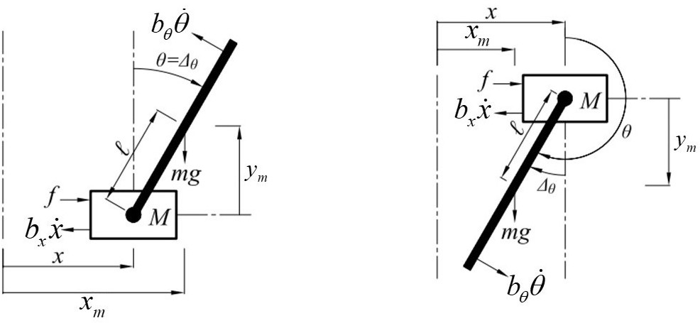
Let x be the horizontal cart displacement and θ be the pendulum angle from the upright vertical. The cart-pendulum configuration and the corresponding coordinate definitions are illustrated in Fig. 1. The Euler–Lagrange equations are shown in (1) and (2):

Here M and m are the cart and pendulum masses; l is the pivot-to-centre-of-mass distance; J is the pendulum inertia; b₁ and b₂ are viscous friction coefficients; g is gravitational acceleration; and F is the cart-driving force. shows the model coordinates.

To relate the driving force to the applied motor voltage u, the armature-current and belt-drive relation is written in (3),

1. Cart–pendulum model and coordinate definition

1. Linearised State-Space Model

The measurable state vector is shown in (4),

The nonlinear model ξ̇ = f(ξ, u) is retained as the simulation plant. For regulator synthesis, it is linearised (in (5)) around ξ = 0 and u = 0, where sin θ ≈ θ and cos θ ≈ 1:

The continuous pair is discretised by a zero-order hold at a sampling period of 0.02 s to obtain the discrete matrices Ad and Bd through MATLAB function in (6),

where T is sample time.

3. Discrete LQR Design

1. Controllability

The linearised pair is controllable when the controllability matrix has rank four in (7):

The condition is satisfied for the nominal parameter set, so a full-state feedback law can be designed.

2. Quadratic Criterion and Gain

The regulator minimises the discrete infinite-horizon cost in (8):

where Q penalises state deviations and R penalises input effort. The control law and Riccati-based gain are shown in (9) and (10),

Q is restricted to a diagonal matrix, leaving four state penalties q₁ to q₄ and one scalar input penalty r. Increasing a state penalty generally speeds the associated response but raises control effort; increasing r makes the input smoother but tends to slow the response.

4. PSO-Based Weight Tuning

1. Encoding and Objective

Each PSO particle represents the diagonal-weight vector in (11),

For every candidate, Q and R are assembled, the discrete Riccati equation is solved, and the nonlinear closed loop is simulated. The PSO fitness is the accumulated sum of squared cart-position tracking errors (SSE), J_SSE = Σ[k=0 to N−1] (x_ref[k] − x[k])². Thus, PSO minimises only the cart-position SSE over the stated simulation horizon. Pendulum-angle deviation, control-voltage demand, settling time, and overshoot are deliberately excluded from J_SSE (in (12)); they are evaluated after optimisation as separate response-quality and feasibility indicators. A candidate that does not yield a finite stabilising Riccati solution or produces a divergent nonlinear response is assigned a large
penalty cost.

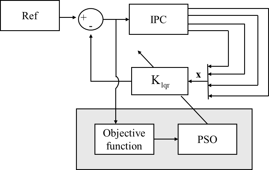
Fig. 2 illustrates the PSO-tuned LQR workflow. The PSO block proposes a candidate vector of diagonal Q and R weights, the LQR block solves the discrete Riccati equation to obtain the feedback gain K, and the nonlinear plant evaluates the resulting closed-loop response. The measured states are returned to the feedback loop, while the fitness block compares the simulated trajectories with the reference and sends the cost back to PSO. Iterations continue until the swarm reaches the selected stopping criterion; the best particle is then used as the final controller.

2. PSO-tuned LQR structure

1. Particle Update

In (13), PSO velocity update combines inertia, attraction to the personal best, and attraction to the global best:

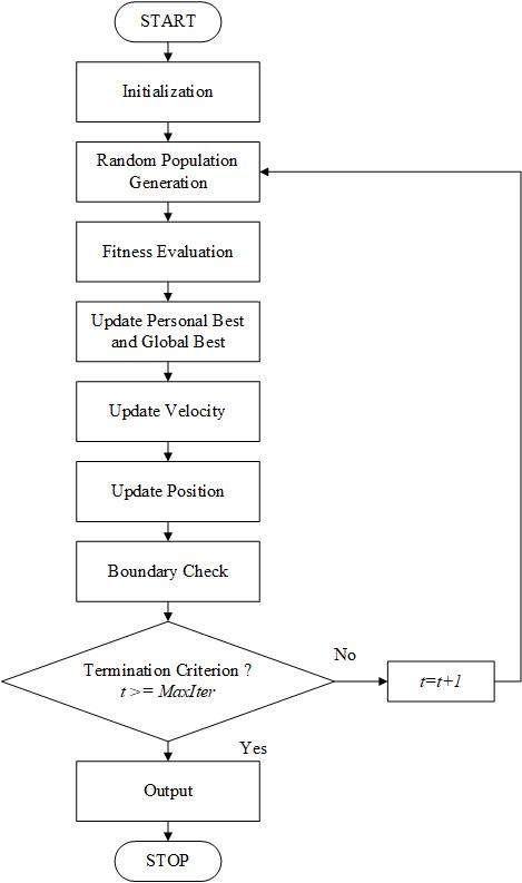
The position is then updated by pᵢ ← pᵢ + vᵢ. The learning coefficients are c₁ = 2.4 and c₂ = 2.22. Candidate weights are bounded as listed, and a divergent simulation receives a large penalty. The PSO uses a swarm of 200 particles and a maximum of 50 iterations. It may terminate earlier when the global-best cart-position SSE no longer decreases in the next iteration (in Table 1). The inertia weight is initialised at w = 1 and reduced using wdamp = 0.92. The same nonlinear plant, 10 s horizon, 0.02 s sample period, initial condition, reference signal, and penalty rule are used for every candidate and every repeated run. Fig. 3 summarises the procedure. The iterative search procedure is shown in Fig. 4.

1. PSO Parameters

3. PSO procedure

The final PSO solution is q₁ = 20048.65, q₂ = 0.2, q₃ = 0.16, q₄ = 166.9001, and r = 0.001. It yields

5. Simulation Setup

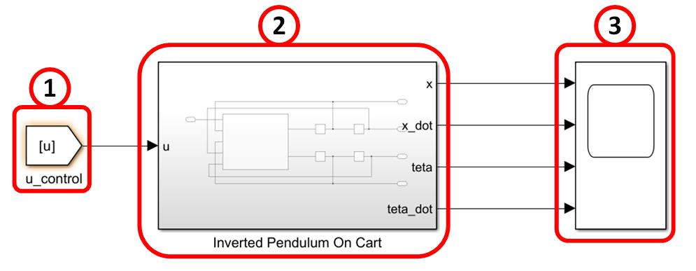
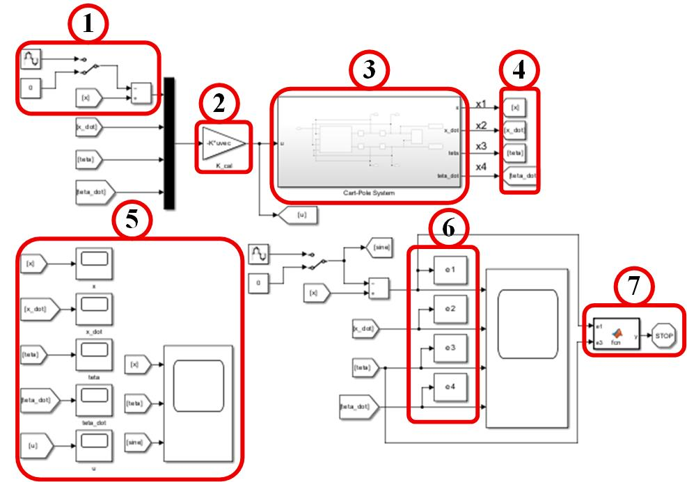
The nonlinear plant is implemented in MATLAB/Simulink using a MATLAB Function block and continuous integrators. The controller can therefore be evaluated against the nonlinear equations rather than only against the linear design model. Fig. 4 shows the nonlinear plant model, whereas Fig. 5 shows the complete closed-loop configuration.

In Fig. 3, block 1 receives the control voltage u_control, block 2 evaluates the nonlinear inverted-pendulum equations and outputs the four states, and block 3 displays the simulated responses for inspection.

4. Simulink realisation of the nonlinear plant

The numbered blocks in Fig. 5 have the following roles: block 1 selects and shapes the cart reference; block 2 computes the tracking error or reference offset; block 3 is the nonlinear cart-pendulum plant; block 4 groups the measured state signals; block 5 supplies the initial conditions and reference profiles; block 6 applies the state-feedback gain K to form the control command; and block 7 sends the command and measured outputs to the monitoring scope. Together, these blocks close the simulation loop from reference generation to plant response and feedback.

5. Closed-loop simulation with reference selection and state feedback

Every simulation uses a 10 s horizon and a 0.02 s sample period. Unless noted otherwise, x(0) = 0.2 m, θ(0) = 0.5236 rad, and both velocity states are zero. The 30° initial tilt tests the practical robustness of a controller designed from a local linearisation. The commanded motor voltage is limited in the simulation to ±48 V, representing the assumed drive-supply limit. This saturation is applied before the plant input; consequently, the reported voltage peaks are interpreted with respect to this assumed limit rather than as experimentally validated actuator requirements. System parameters in simulink in shown in Table 2. The nominal plant parameters used in these simulations are listed in Table 2.

2. Nominal Parameters of the Simulated Plant

6. Simulation Results

1. Upright-Equilibrium Regulation

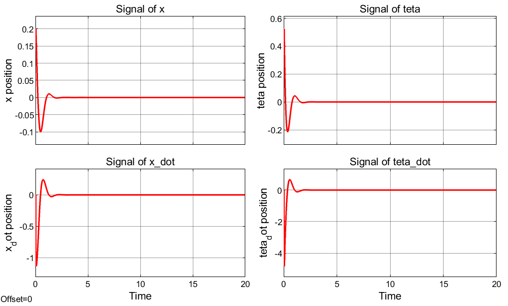
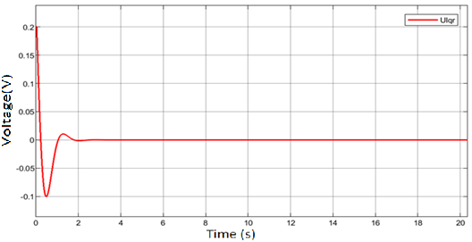
With the reference held at zero, the PSO-LQR gain drives the cart from 0.2 m to the origin and returns the pendulum from 30° to the upright position. The cart undershoots to approximately −0.10 m before converging. The settling times are 2.22 s for the cart and 2.20 s for the pendulum. The saturated command reaches a peak of 40.53 V and decays to zero in 3.92 s. This peak is below the assumed ±48 V drive limit, but it is close enough to the limit that hardware implementation would require actuator-margin verification. Fig. 6 shows the state trajectories, and Fig. 7 shows the command voltage. Table 3 summarises the regulation performance and weight sensitivity.

6. State trajectories during upright-equilibrium regulation

7. Command voltage during regulation

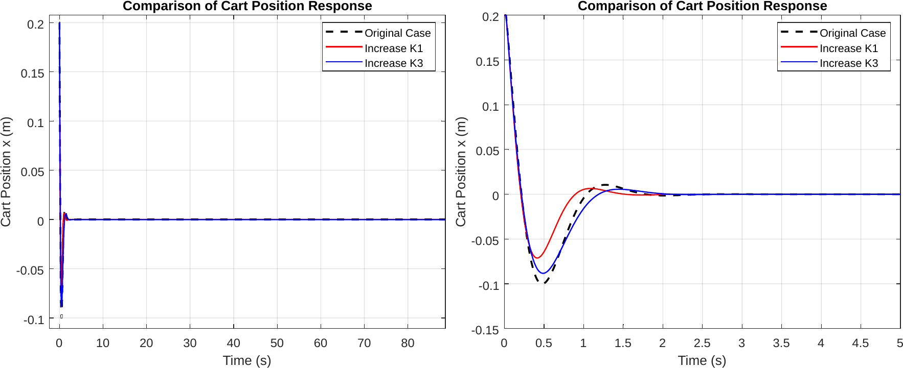
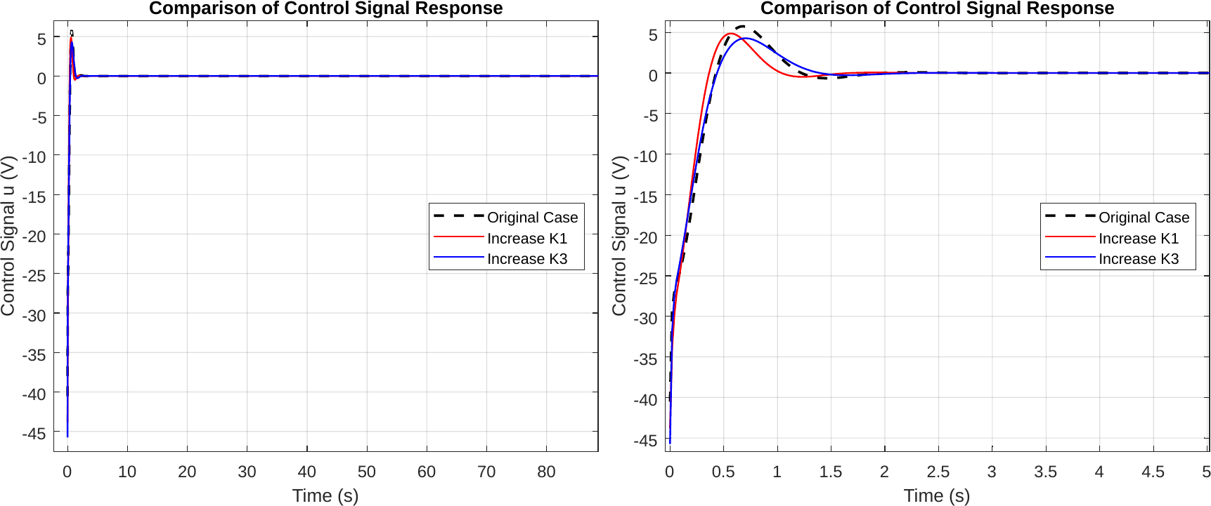
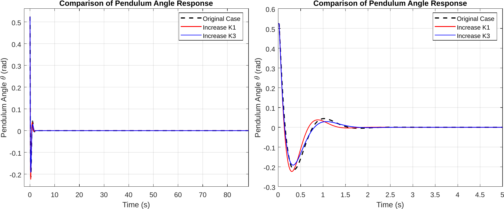
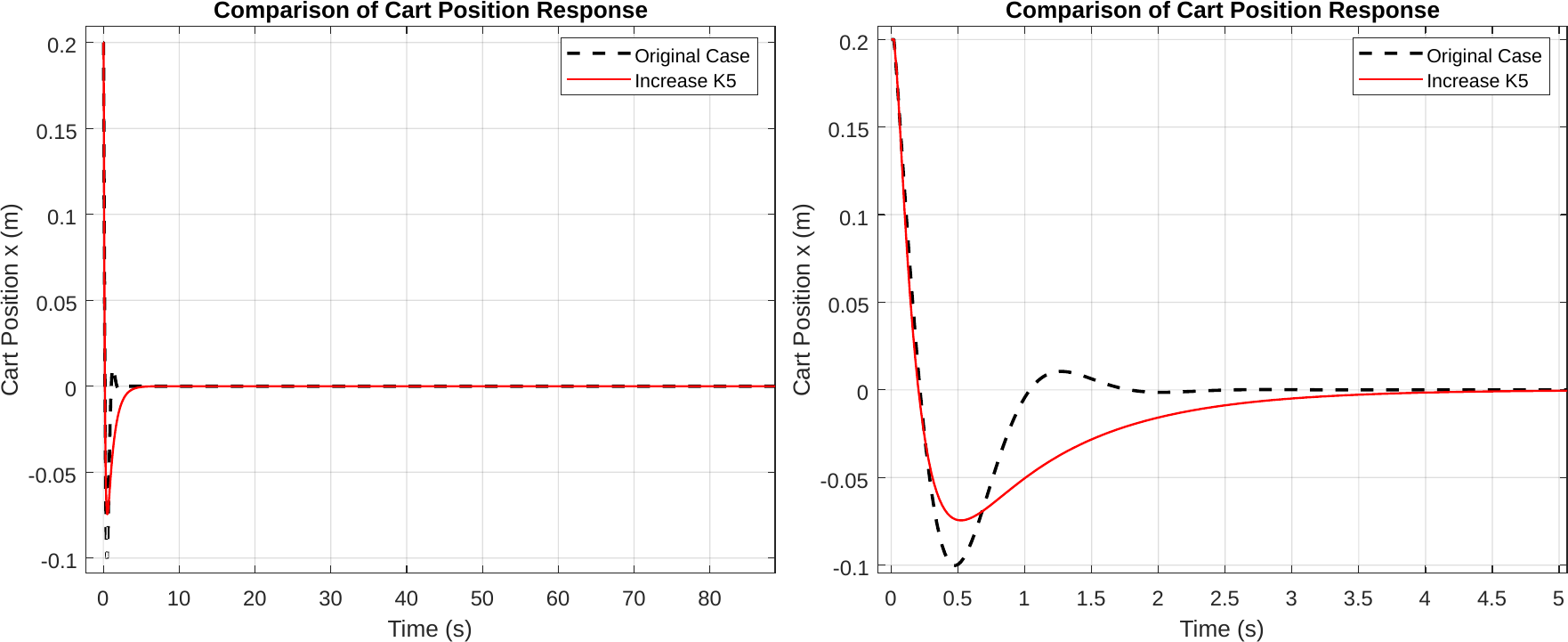
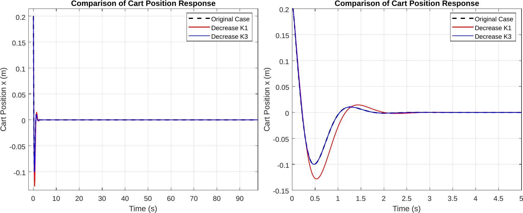
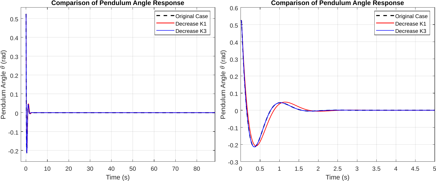
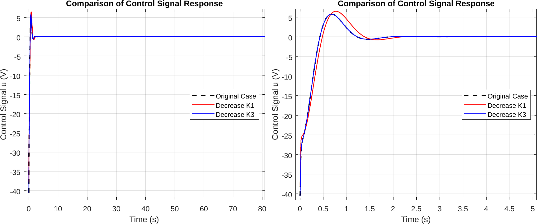
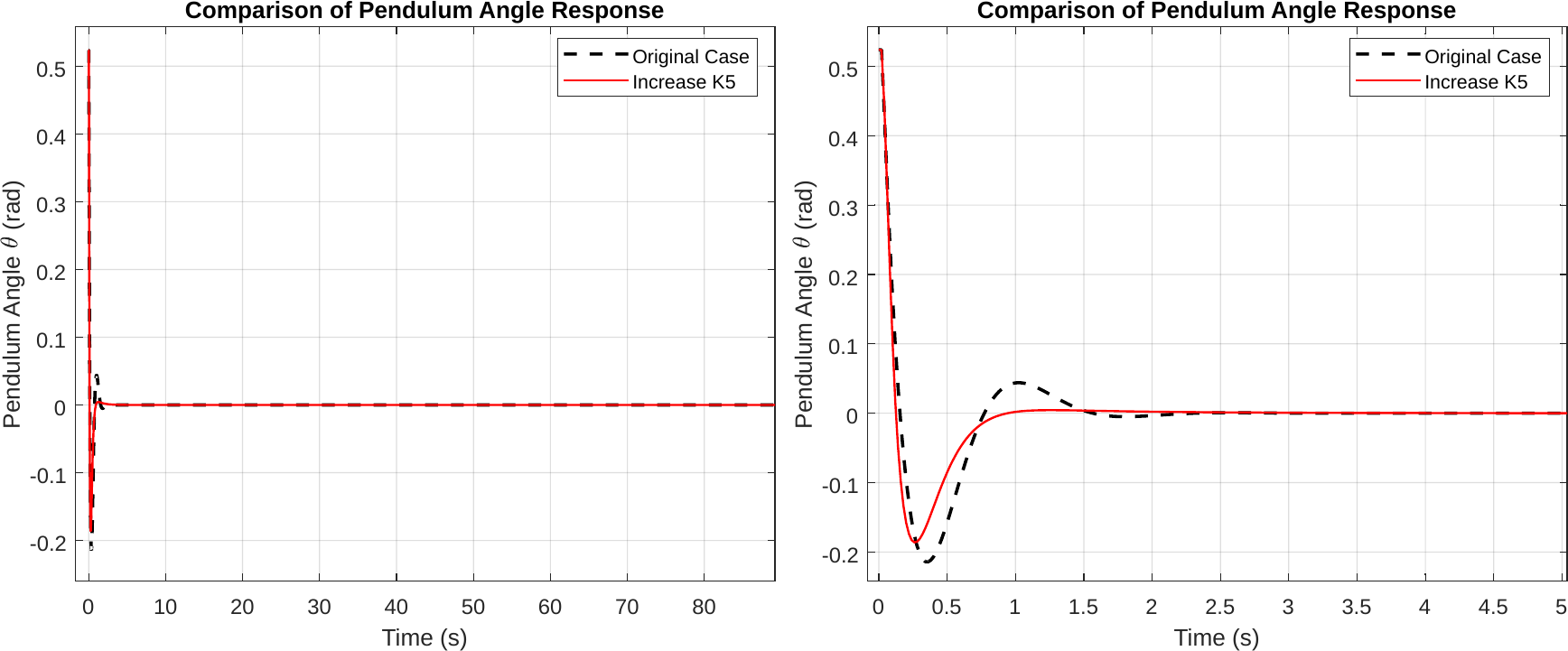
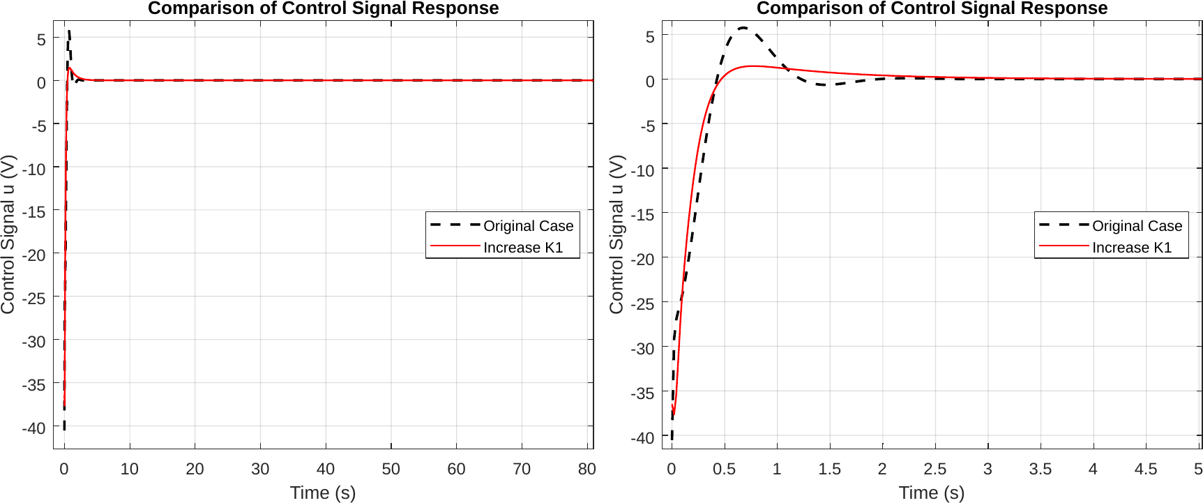
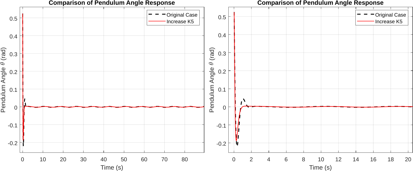
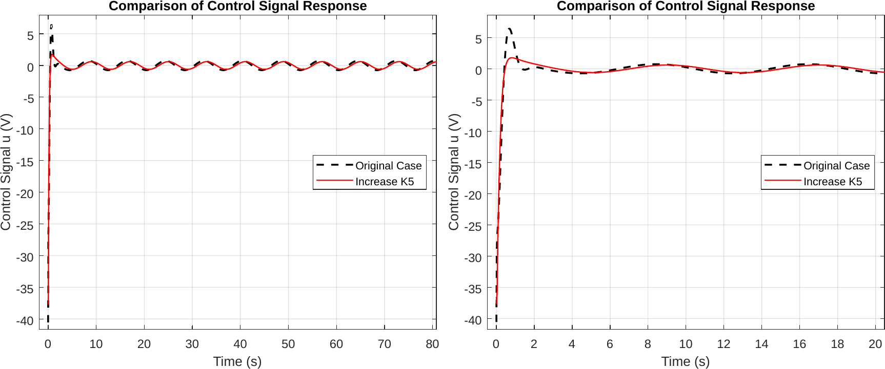
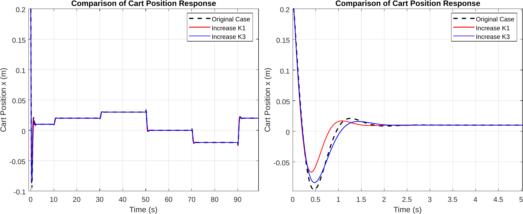
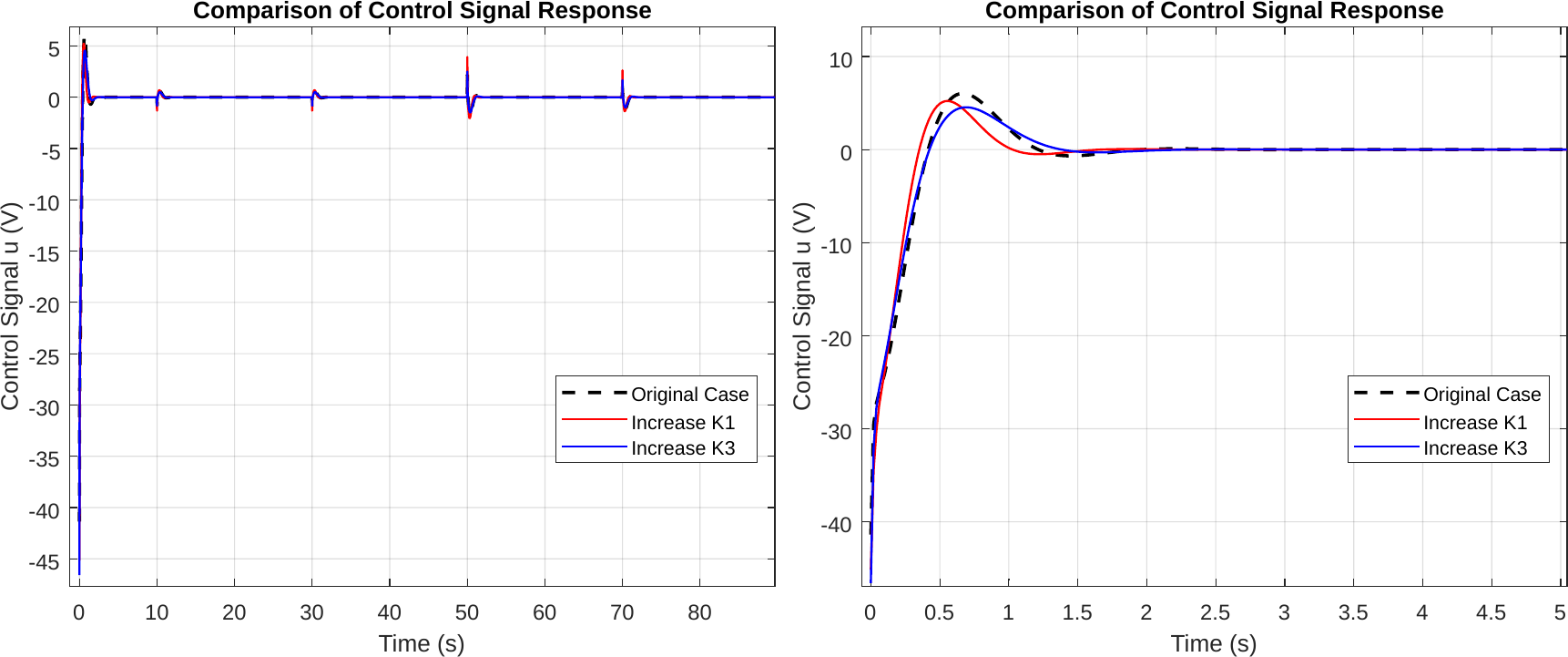
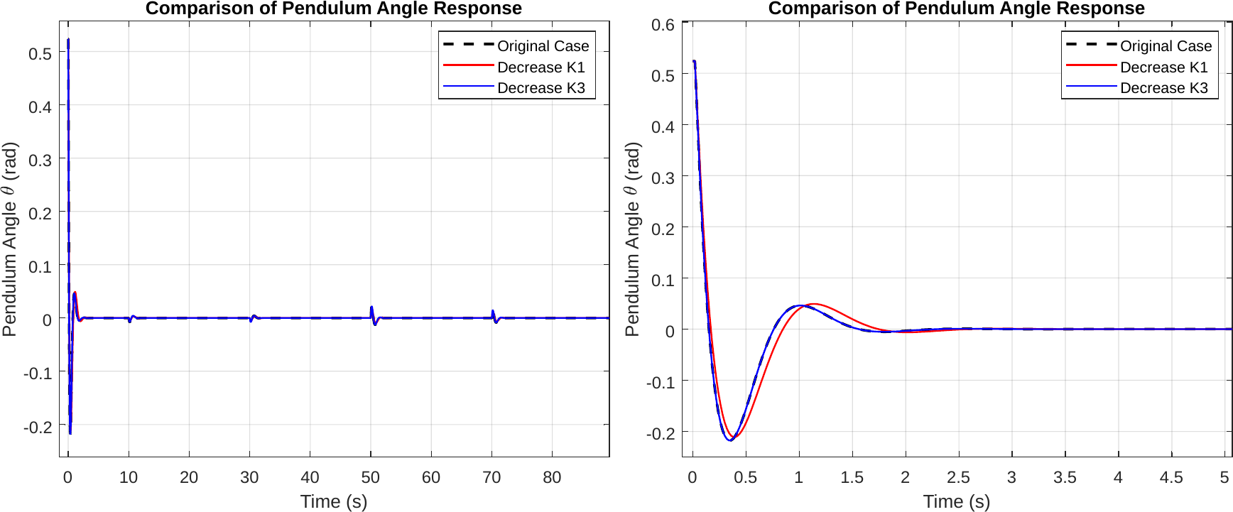
Fig. 8 compares the cart-position responses for the raised-Q cases during regulation. Fig. 9 compares their control voltages. Fig. 10 compares the associated pendulum-angle responses. Fig. 11 shows the control-voltage response for the raised-R case. Fig. 12 compares cart-position responses for the lowered-Q cases, while Fig. 13 compares their pendulum-angle responses and Fig. 14 compares their control voltages. Fig. 15 compares cart-position responses for the raised-R cases, and Fig. 16 compares their control voltages. Together, these figures make the effect of the changed state and input penalties explicit.

3. Regulation Performance and Weight Sensitivity

8. Cart-position comparison for the raised-Q cases during regulation

9. Control-voltage comparison for the raised-Q cases during regulation

10. Pendulum-angle comparison for the raised-Q cases during regulation

11. Control-voltage comparison for raised-R cases during regulation

12. Cart-position comparison for lowered-Q cases during regulation

13. Pendulum-angle comparison for lowered-Q cases during regulation

14. Control-voltage comparison for lowered-Q cases during regulation

15. Cart-position comparison for raised-R cases during regulation

16. Control-voltage comparison for raised-R cases during regulation

Increasing q₁ makes both state responses faster and reduces SSE, but raises the peak command. Increasing q₃ produces a stronger pendulum action and the largest control demand. Raising r reduces the peak voltage but nearly doubles the cart settling time, confirming the speed-versus-effort trade-off.

2. Sinusoidal Tracking

For sinusoidal tracking, a 0.04 m position command with a 0.02 s sample time is applied after the pendulum is brought upright. Since a continuously varying reference has no final settling value, performance is measured using (15).

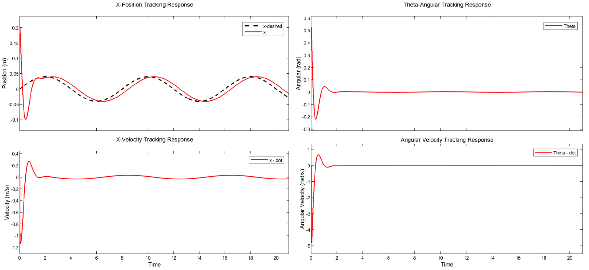
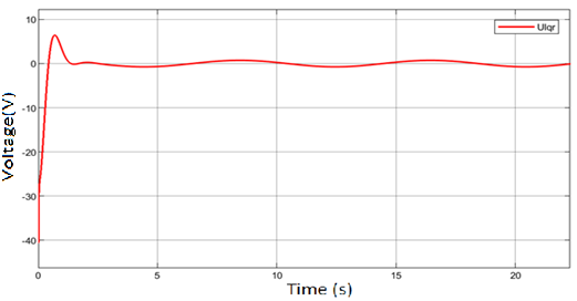
The baseline achieves RMS errors of 0.012519 m in cart position and 0.013005 rad in pendulum angle. The cart follows the reference after the initial transient, while the pendulum remains within a few hundredths of a radian of vertical. Fig. 17 shows the state trajectories, Fig. 18 shows the command-voltage response, and Table 4 reports the RMS-error values.

17. State trajectories during sinusoidal reference tracking

18. Command voltage during sinusoidal tracking

4. Sinusoidal-Tracking RMS Errors

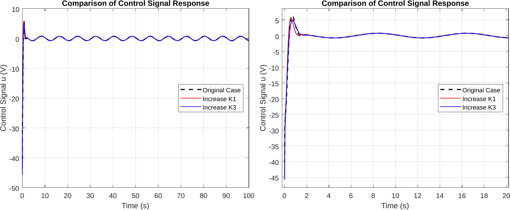
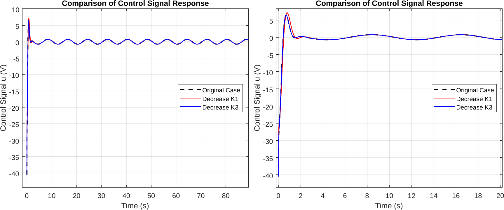
Fig. 19 compares cart-position responses for the raised-Q cases during sinusoidal tracking. Fig. 20 compares their control voltages, and Fig. 21 compares their pendulum-angle responses. Fig. 22 compares cart-position responses for the raised-R case. Fig. 23 compares cart-position responses for the lowered-Q cases, Fig. 24 compares their pendulum-angle responses, and Fig. 25 compares their control voltages.
Fig. 26 compares the pendulum-angle response for the raised-R case, while Fig. 27 compares its control-voltage response. These comparisons show that a larger q₁ reduces the position-error envelope without destabilising the angular loop, whereas a larger q₃ alters the angular transient more directly and requires a visibly more active command.

19. Cart-position comparison for raised-Q cases during sinusoidal tracking

20. Control-voltage comparison for raised-Q cases during sinusoidal tracking

21. Pendulum-angle comparison for raised-Q cases during sinusoidal tracking

22. Cart-position comparison for raised-R cases during sinusoidal tracking

23. Cart-position comparison for lowered-Q cases during sinusoidal tracking

24. Pendulum-angle comparison for lowered-Q cases during sinusoidal tracking

25. Control-voltage comparison for lowered-Q cases during sinusoidal tracking

26. Pendulum-angle comparison for raised-R cases during sinusoidal tracking

27. Control-voltage comparison for raised-R cases during sinusoidal tracking

The sinusoidal plots also reveal the different roles of the two state penalties. The raised-q₁ response reduces the cart-position error envelope almost immediately after each reversal of the reference, while the angular trace remains close to the baseline trace. This indicates that the additional position penalty is absorbed mainly by cart acceleration rather than by a large pendulum excursion.

The raised-q₃ case produces a more pronounced correction in the first cycles. Its pendulum angle returns to the upright region quickly, but the corresponding command-voltage trace contains sharper peaks. In practical tuning terms, q₃ is therefore useful when angular protection is the priority, although the improvement is obtained at the expense of actuator activity.

The lowered-Q plots provide an important robustness check. Reducing q₁ or q₃ does not cause instability in the simulated plant, but it increases the residual tracking envelope and makes the transient less decisive. The response remains bounded because the nominal gain retains a stabilising margin, yet the figures show that a lower-cost design is not automatically a better tracking design.

For this moving-reference case, increasing q₁ improves both cart and angle tracking. In contrast, increasing r almost doubles the cart RMS error because the controller becomes too conservative to follow a continuously changing command.

3. Staircase-Reference Tracking

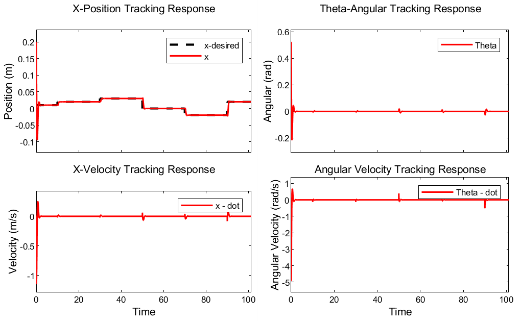
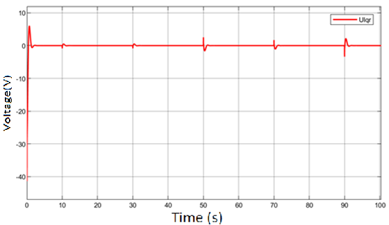
The staircase command moves the cart through approximately 0.02 m, 0.03 m, 0 m, −0.02 m, and back to 0.02 m. The cart settles within approximately 1–2 s after each transition with negligible steady-state offset. The pendulum converges from 0.5236 rad in about 2 s and remains within approximately ±0.02 rad during command changes. Fig. 28 shows the state trajectories, Fig. 29 shows the command-voltage response, and Table 5 reports the staircase-tracking performance and weight sensitivity.

28. State trajectories during staircase-reference tracking

Fig. 30 compares cart-position responses for the raised-Q cases during staircase tracking. Fig. 31 compares their pendulum-angle responses, and Fig. 32 compares their control-voltage responses. Fig. 33 compares cart-position responses for the lowered-Q cases, Fig. 34 compares their pendulum-angle responses, and Fig. 35 compares their control-voltage responses. Fig. 36 compares cart-position responses for the raised-R case, Fig. 37 compares its pendulum-angle response, and Fig. 38 compares its control-voltage response. The most aggressive setting is q₃ raised, which reaches the largest command excursion of 46.58 V. This value remains below the assumed ±48 V saturation limit, although its small margin indicates that this tuning would be sensitive to a lower available supply voltage or unmodelled actuator losses.

29. Command voltage during staircase tracking

5. Staircase-Tracking Performance and Weight Sensitivity

30. Cart-position comparison for raised-Q cases during staircase tracking

31. Pendulum-angle comparison for raised-Q cases during staircase tracking

The staircase figures make the transient trade-offs easier to distinguish than the sinusoidal case. At each step, the q₁-raised controller reaches the new cart position with a shorter excursion, whereas the q₃-raised controller prioritises a rapid reduction of the angular error. The reference levels themselves are reproduced by all cases, so the main differences appear in overshoot, settling time, and command amplitude.

32. Control-voltage comparison for raised-Q cases during staircase tracking

33. Cart-position comparison for lowered-Q cases during staircase tracking

34. Pendulum-angle comparison for lowered-Q cases during staircase tracking

35. Control-voltage comparison for lowered-Q cases during staircase tracking

For the raised-R case, the cart trajectory changes more gradually after every step and the command signal is visibly smoother. This behaviour is desirable when actuator saturation or mechanical wear is a concern, but the longer transient means that the cart spends more time away from the requested position. The comparison therefore supports using r as an effort-limiting parameter after acceptable tracking speed has been established.

Across the angle plots, the pendulum remains within a small neighbourhood of zero after the initial recovery. The absence of growing oscillations in the regulation, sinusoidal, and staircase records is evidence that the nonlinear simulation remains stable for the tested references. It does not, however, establish stability for untested disturbances or for a physical implementation.

36. Cart-position comparison for raised-R cases during staircase tracking

37. Pendulum-angle comparison for raised-R cases during staircase tracking

38.  Control-voltage comparison for raised-R cases during staircase tracking

1. Cross-Scenario Discussion

The same pattern appears in the regulation, sinusoidal, and staircase tests. Of the state weights, q₁ has the clearest effect on cart motion: increasing it shortens the transient and reduces the tracking error, but the initial recovery and each reference change require more voltage. Thus, q₁ is the most direct parameter to adjust when a faster cart response is needed.

Changing q₃ mainly affects the pendulum angle. A larger q₃ makes the controller correct angular deviations more aggressively and produces the largest voltage peaks. Reducing q₃, on the other hand, changes the responses only slightly around the PSO solution. In this region, the optimisation appears to have found a relatively insensitive set of smaller q₃ values.

The weight r controls how much input effort the controller is willing to use. Raising r smooths the command and lowers its peak in all three tests, but the slower response is especially visible for the sinusoidal reference. A controller that is too cautious cannot follow a continuously moving target without increasing the position error.

These results also show why SSE is not interpreted as a complete control-quality measure. SSE is intentionally used only as the PSO fitness because it gives a clear and directly reproducible tracking criterion. The response tables and figures separately report settling time, pendulum-angle response, overshoot, and voltage demand. For example, the raised-r case can achieve a lower regulation SSE while taking considerably longer to settle. A low-SSE solution must therefore still be screened against the independent transient and actuator indicators.

Overall, the q₁-raised setting gives a faster response at the cost of higher voltage, while the r-raised setting reduces actuator effort but slows the motion. The q₃-raised setting is the most demanding for the actuator, with a peak voltage of 46.58 V. These conclusions describe the tested nonlinear simulations only.

7. Conclusion

A PSO-tuned discrete LQR controller was designed for the nonlinear inverted-pendulum-on-a-cart model and evaluated exclusively in MATLAB/Simulink. The PSO fitness was the cart-position sum of squared errors (SSE); pendulum-angle response, settling time, overshoot, and control voltage were not optimisation terms and were instead used as post-optimisation evaluation indicators. This distinction makes the optimisation objective consistent across the abstract, method, and results. The selected gain stabilises a 30° initial tilt in approximately 2.2 s and tracks sinusoidal and staircase cart references while keeping the pendulum close to upright.

The simulation sensitivity study identifies the cart-position weight q₁ as the most effective single tuning parameter. The input penalty r gives a clear trade-off between control effort and tracking speed. The largest reported command, 46.58 V, remains below the assumed ±48 V saturated drive limit, but this margin should be verified for any physical actuator. These conclusions apply to the stated nonlinear simulation model; no experimental or hardware-implementation claims are made in this manuscript.

Acknowledgement

This research was funded by Ho Chi Minh City University of Technology and Engineering, Vietnam, under grant No. SV2026- 236. We want to give thanks to Ph.D. Van-Dong-Hai Nguyen (HCM-UTE) due to his supervision.

References

1. D.-P. Hoang et al., “A Survey of Experimental LQR for Cart and Pole,” Journal of Fuzzy Systems and Control, vol. 2, no. 2, pp. 97–103, 2024, https://doi.org/10.59247/jfsc.v2i2.211.
2. L. B. Prasad, B. Tyagi, and H. O. Gupta, “Optimal Control of Nonlinear Inverted Pendulum System Using PID Controller and LQR: Performance Analysis Without and With Disturbance Input,” International Journal of Automation and Computing, vol. 11, no. 6, pp. 661–670, 2014, https://doi.org/10.1007/s11633-014-0818-1.
3. V. Radisavljevic-Gajic, “Linear–quadratic optimal steady state controllers for engineering students and practicing engineers,” International Journal of Mechanical Engineering Education, vol. 49, no. 4, pp. 316–358, 2021, https://doi.org/10.1177/0306419019876109.
4. E. Vinodh Kumar and J. Jerome, “Robust LQR controller design for stabilizing and trajectory tracking of inverted pendulum,” Procedia Engineering, vol. 64, pp. 169–178, 2013, https://doi.org/10.1016/j.proeng.2013.09.088.
5. J. Kennedy and R. Eberhart, “Particle swarm optimization,” in Proceedings of ICNN’95 - International Conference on Neural Networks, Perth, Australia: IEEE, 2013, pp. 1942–1948, https://doi.org/10.1109/ICNN.1995.488968.

6. Y. Shi and R. Eberhart, “A modified particle swarm optimizer,” in 1998 IEEE International Conference on Evolutionary Computation Proceedings. IEEE World Congress on Computational Intelligence (Cat. No.98TH8360), Anchorage, AK, USA: IEEE, 1998, pp. 69–73, https://doi.org/10.1109/ICEC.1998.699146.
7. S. Howimanporn, S. Thanok, S. Chookaew, and W. Sootkaneung, “Design and implementation of PSO based LQR control for inverted pendulum through PLC,” in 2016 IEEE/SICE International Symposium on System Integration (SII), Sapporo, Japan: IEEE, pp. 664–669, 2026, 2016, https://doi.org/10.1109/SII.2016.7844075.
8. J.-J. Wang, “Simulation studies of inverted pendulum based on PID controllers,” Simulation Modelling Practice and Theory, vol. 19, no. 1, pp. 440–449, 2011, https://doi.org/10.1016/j.simpat.2010.08.003.
9. A. Kharola, P. Patil, S. Raiwani, and D. Rajput, “A comparison study for control and stabilisation of inverted pendulum on inclined surface (IPIS) using PID and fuzzy controllers,” Perspectives in Science, vol. 8, pp. 187–190, 2016, https://doi.org/10.1016/j.pisc.2016.03.016.
10. T. Abut, “An Inverted Pendulum System Control with Fuzzy Linear Quadratic Regulator Method: Experimental Validation,” Computers, Materials & Continua, vol. 85, no. 2, pp. 4023–4042, 2025, https://doi.org/10.32604/cmc.2025.066920.

11. M. Ali and S. Mandal, “Preparation of Papers for IFAC Conferences & Symposia: Kalman Filter Based Control of Inverted Pendulum System,” IFAC-PapersOnLine, vol. 55, no. 1, pp. 58–63, 2022, https://doi.org/10.1016/j.ifacol.2022.04.010.
12. S. J. Chacko, P. C. Neeraj, and R. J. Abraham, “Optimizing LQR controllers: A comparative study,” Results in Control and Optimization, vol. 14, p. 100387, 2024, https://doi.org/10.1016/j.rico.2024.100387.
13. Y. Qu, Z. Liu, and L. Cai, “Simultaneous planning and executing (SPAE) control for a fourth-order underactuated inverted pendulum with double-layer asynchronous convergence,” ISA Transactions, vol. 163, pp. 162–171, 2025, https://doi.org/10.1016/j.isatra.2025.05.004.
14. Q. Zhu, C. Lei, B. Shi, J. Zhang, and J. Wang, “Model-free robust underactuated control of inverted pendulums,” Journal of the Franklin Institute, vol. 362, no. 13, p. 107911, 2025, https://doi.org/10.1016/j.jfranklin.2025.107911.
15. A. H. Bajodah and U. Ansari, “Rotary Inverted Pendulum Control using Robust Generalized Dynamic Inversion with Adaptive Neural Estimation,” IFAC-PapersOnLine, vol. 56, no. 2, pp. 10570–10575, 2023, https://doi.org/10.1016/j.ifacol.2023.10.675.
16. Y. E. Bezci et al., “Classical and intelligent methods in model extraction and stabilization of a dual-axis reaction wheel pendulum: A comparative study,” Results in Engineering, vol. 16, p. 100685, 2022, https://doi.org/10.1016/j.rineng.2022.100685.