Hybrid Multilayer Perceptron and Grey Wolf Optimization Model for Peak Load Forecasting

Rudi Yusmawarsyah 1, *, Ramdhan Halid Siregar 2, Zulfikar Zulfikar 3, Roslidar Roslidar 4, Tarmizi Tarmizi 5

Department of Electrical and Computer Engineering, Universitas Syiah Kuala, Aceh, Indonesia

Email: rudi.yusmawarsyah@gmail.com

*Corresponding Author

Abstract—The growth of electrical energy consumption continues to increase, particularly during peak-load periods, posing significant challenges to power system reliability. Inaccurate peak-load forecasting can lead to supply–demand imbalances, reduced power plant operational efficiency, and an increased risk of power outages. This study aims to develop a machine learning-based peak-load forecasting model by integrating a Multilayer Perceptron (MLP) with the Grey Wolf Optimizer (GWO) algorithm to achieve more accurate and stable forecasting performance. The dataset consists of historical electricity load data collected from January 2024 to January 2025 and is supplemented with relevant weather variables. The proposed model is evaluated using Mean Squared Error (MSE), Root Mean Squared Error (RMSE), Mean Absolute Error (MAE), and Mean Absolute Percentage Error (MAPE). The results demonstrate that the integrated MLP–GWO model achieves improved forecasting performance compared with the standard MLP, attaining a MAPE of 0.69%. The findings indicate that GWO-based optimization improves convergence and model stability while enhancing the ability of the MLP to capture nonlinear patterns in daily peak-load demand. Therefore, the proposed MLP–GWO model provides an effective approach for peak-load forecasting and can support power system planning, including generation capacity assessment, distribution network reinforcement, and renewable energy integration, thereby contributing to a more reliable and sustainable electricity system.

Keywords—Electricity Demand; Grey Wolf Optimizer; Machine Learning; Multilayer Perceptron; Peak-Load Forecasting

1. Introduction

Electricity demand in Indonesia, including in Banda Aceh, has shown a consistent upward trend in line with population growth, economic development, and urbanization. As a center of government, education, and commerce, Banda Aceh has experienced a significant increase in electricity consumption, particularly during peak load periods. Peak load conditions are crucial because they are directly related to the reliability and efficiency of the power system. Inaccurate peak load forecasting can cause imbalances between supply and demand, reduce power plant operational efficiency, and potentially lead to power outages that adversely affect both the community and economic activities [1], [2].

Traditional approaches such as linear regression, Autoregressive Integrated Moving Average (ARIMA), and similar statistical models are still widely used for peak load forecasting. However, these methods exhibit limitations in capturing the nonlinear and complex patterns inherent in peak load behavior [2]. Electrical load data are influenced by various external factors, including weather conditions, calendar patterns, and human activities. These factors are often difficult to model accurately using purely statistical techniques. This situation highlights the need to develop peak load forecasting models based on Machine Learning (ML). ML methods are considered more adaptive and capable of generalizing nonlinear and complex patterns effectively.

One of the promising ML methods for developing a peak load forecasting model is the MLP. MLP can learn nonlinear patterns in time-series data [3].  However, its predictive accuracy is highly dependent on the choice of network parameters, particularly the initial weights and biases. Improper parameter initialization may lead the network to fall into local minima or suffer from suboptimal convergence. To address this issue, an optimization technique is required to systematically determine the best initial weight and bias configuration. In this study, the GWO is specifically employed to globally optimize the initial weights and biases of a predefined MLP architecture. The structural hyperparameters, including the number of hidden neurons (fixed at 16), the learning rate (fixed at 0.001 using the Adam optimizer), and the training epochs (evaluated at 100 and 200) are kept constant throughout the optimization process and are not decision variables for GWO [3].

Various studies integrating MLP and GWO have demonstrated positive results. Research in [4] showed that the combination of MLP and GWO achieves higher accuracy compared to a standalone MLP model or the Adaptive Neuro-Fuzzy Inference System (ANFIS) in predicting solar diffuse fraction [5]. In the context of energy prediction for microgrid systems, the integration of GWO with Random Forest has produced high accuracy, with RMSE values ranging from 0.03 to 0.05. For long-term electricity load forecasting, the combination of GWO and Least Squares Support Vector Machine (LSSVM) outperformed other methods, achieving a MAPE of 0.13% [5]. Additionally, the contribution of GWO has also shown positive outcomes in optimizing load frequency control devices in micro-hydropower plants, effectively enhancing system stability against load fluctuations [6].

Based on the above studies, the MLP–GWO approach consistently delivers more accurate forecasting results compared to other methods. However, its application has remained limited to large-scale and wide-area power systems. Therefore, this study aims to introduce a new contribution by applying the MLP and GWO hybrid model for peak load forecasting in Banda Aceh, thereby expanding the implementation of hybrid models within electrical power systems. This study integrates the MLP architecture with the GWO algorithm to globally optimize the weights and biases of the MLP, thereby overcoming the limitations of conventional training and improving forecasting accuracy. The research focuses on energy consumption during peak load hours in Banda Aceh. By employing the hybrid MLP–GWO model, this approach offers a more computationally lightweight alternative compared to complex deep learning architectures, while remaining robust in handling nonlinear and fluctuating patterns. This enables the development of a more precise peak-load forecasting model. This integrative approach is expected to produce a forecasting model that is not only more accurate but also more efficient in the training process and more adaptive to real-time data dynamics, ultimately supporting more informed decision-making in energy distribution system management. While the MLP–GWO hybrid framework has been explored in general power systems, this study serves as an empirical validation and domain-specific confirmation on localized transformer-level load profiles (TD1, TD2, and TD3) in the Banda Aceh distribution network

In addition, the main contributions of this paper are as follows:

• Proposing a hybrid MLP–GWO model specifically designed for peak load forecasting in Banda Aceh, an application that has not been extensively explored in previous studies.
• Demonstrating enhanced forecasting accuracy on real power system data, showing the capability of the hybrid model to handle nonlinear and highly fluctuating load characteristics.

The rest of the paper is organized as follows: Section 2 presents the related work and theoretical background; Section 3 describes the proposed MLP–GWO methodology; Section 4 discusses the experimental setup and results; and Section 5 concludes the study with key findings and future work.

2. Related Work

The demand for electrical energy in Banda Aceh has shown a consistent growth trend each year, driven by increasing economic activity, urbanization, and the digitalization of public services. However, the irregular and fluctuating nature of electricity consumption patterns presents a significant challenge for load forecasting. Inaccurate load predictions can lead to several serious consequences, including supply–demand imbalances, increased operational burdens and generation costs for PLN, and the risk of system disturbances such as power outages, ultimately affecting the stability and reliability of the electrical power system.

Previous studies have generally relied on conventional approaches such as regression models [7]–[9], time-series methods like ARIMA [10]–[12], or artificial intelligence algorithms that have not been fully optimized, such as standard MLP models [13]–[15]. These approaches exhibit limitations in accommodating the complexity of electrical load data, which are inherently nonlinear and strongly influenced by short-term dynamics, including weather variations, differences between weekdays and holidays, and shifting consumption patterns across industrial and residential sectors. Therefore, a more adaptive and highly accurate forecasting method is required to address these challenges.

Research on the use of MLP architectures for developing electrical load forecasting models has been extensively conducted. Study [16] compares forecasting performance using several methods, including MLP and ARIMA, on the East Java and Bali subsystems. The results show that the MLP architecture provides better accuracy compared to ARIMA-based forecasting models. This finding offers an important foundation for applying MLP architectures to develop load forecasting models on a smaller scale, such as the Banda Aceh region. However, this prior work did not employ any metaheuristic optimization techniques to determine the optimal MLP architecture.

Study [17] developed and compared energy consumption forecasting models using an MLP architecture and regression-based models. The results indicated that the MLP-based model demonstrated superior capability in capturing complex data fluctuations compared to the regression model. Nevertheless, the developed MLP model still exhibited weaknesses during the training phase, particularly in determining optimal network parameters such as initial weights and biases. Inaccuracies in this configuration may lead to overfitting or underfitting, which directly reduces forecasting accuracy.

The study conducted by Insani and colleagues employed a multivariate time-series machine learning approach integrated with an optimization algorithm to develop a household electricity consumption forecasting model [18]. However, the study did not specifically utilize nature-inspired metaheuristic algorithms such as GWO, which are known for their strong capabilities in exploring the solution space and achieving efficient convergence. Husni developed an MLP architecture to construct a short-term load forecasting model based on weekday and holiday classifications in the Aceh power system [19]. The model produced highly positive accuracy results. However, the study relied on a trial-and-error approach to determine the optimal MLP architecture. It did not examine the use of metaheuristic algorithms such as GWO, which could expand the search space for optimal solutions across more complex and globally distributed parameters.

The study in [10] implemented an MLP architecture to develop a short-term electrical load forecasting model. However, the model relied on standard MLP training, which is susceptible to local minima and highly dependent on the initialization of weights. Based on these limitations, the present study integrates the MLP architecture with the GWO algorithm to globally optimize the weights and biases, thereby overcoming the constraints of conventional training and improving forecasting accuracy. This research focuses on energy consumption during peak load hours in Banda Aceh. By employing the hybrid MLP–GWO model, the proposed approach offers a computationally lighter alternative to complex deep learning architectures while remaining robust in handling nonlinear and highly fluctuating patterns, resulting in more precise peak-load forecasting. This integrative approach is expected to produce a forecasting model that is not only more accurate but also more efficient during training and more adaptive to real-time data dynamics, ultimately supporting more informed decision-making in energy distribution system management.

3. Methods

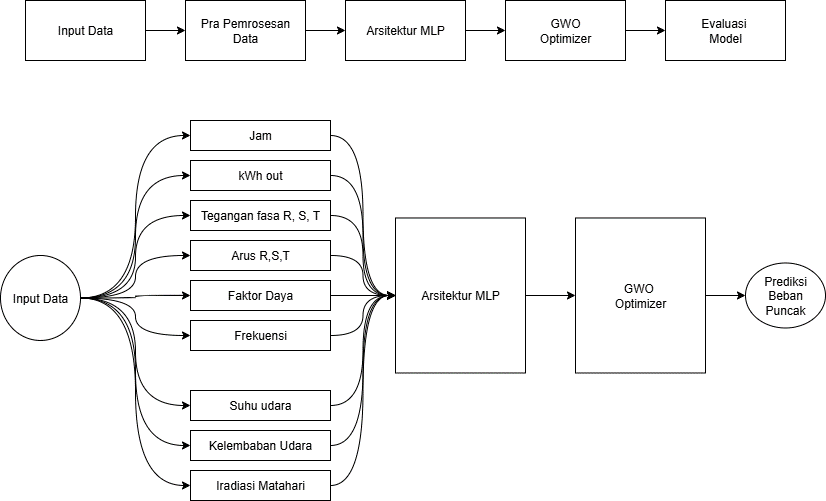
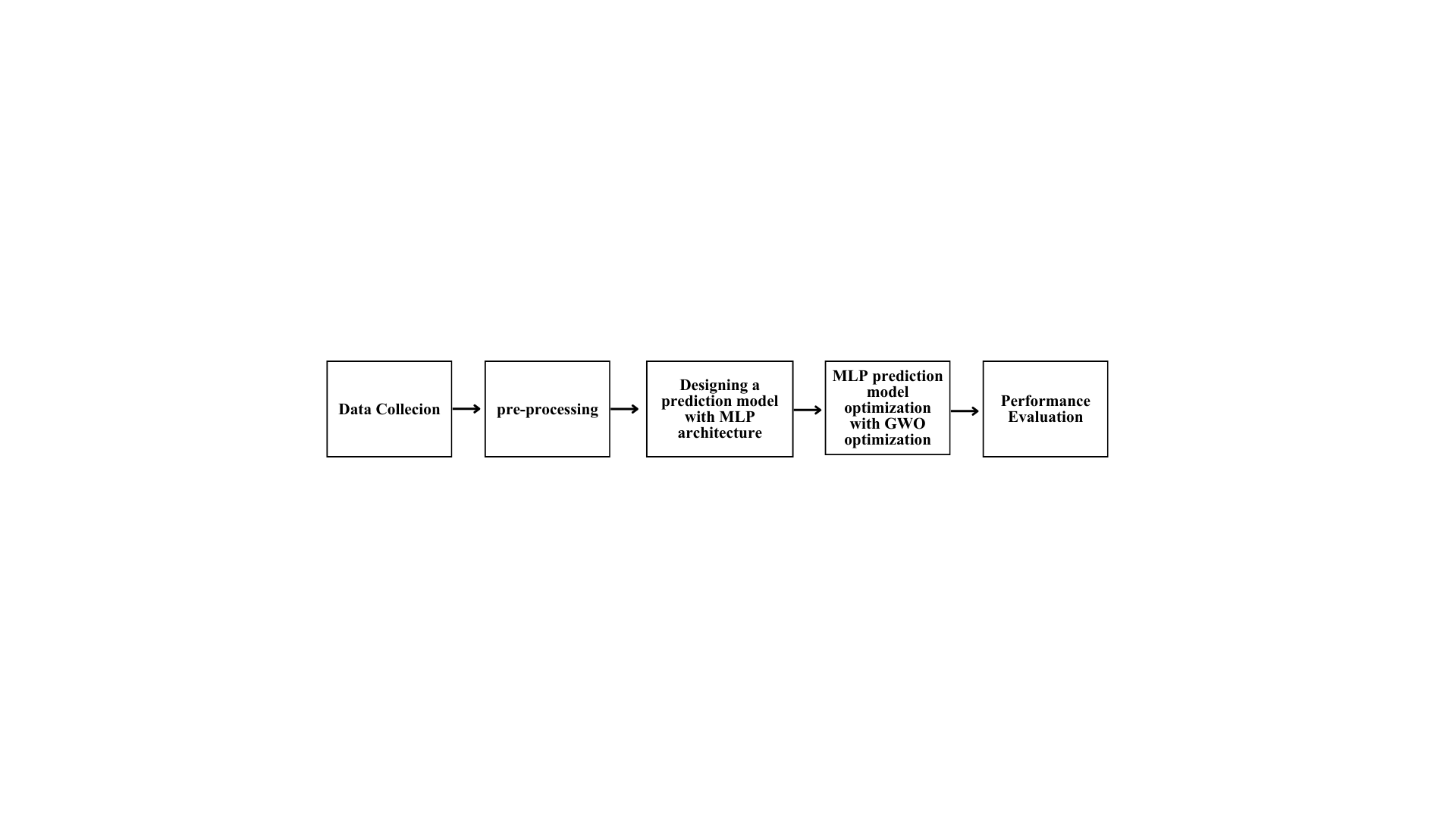
This study was conducted through several systematic steps, as illustrated in Fig. 1. Each stage will be described as follows.

1. The proposed framework

1. Data Collection

The required data consist of historical electrical load data for the city of Banda Aceh, along with 24-hour technical variables recorded at the Lambaro Substation [20]-[22], and NASA POWER Satellite Data. The peak load prediction model is further supported by additional variables, including air temperature, humidity, and solar radiation intensity. Air temperature is selected because it is the most dominant factor influencing electricity consumption. As temperature increases, the use of air conditioning rises significantly, leading to sharp increases in electrical load, especially during peak hours. A similar effect occurs with humidity levels. High humidity intensifies the sensation of heat, which in turn increases the use of cooling systems. This makes humidity an important factor for tropical regions such as Banda Aceh. In addition, solar radiation or sunlight intensity also contributes to increases in electricity demand. High solar radiation during daytime hours drives a greater need for cooling, resulting in a higher electrical load [23]-[24].

The historical electrical load data were collected from three power transformers, which are denoted as TD1, TD2, and TD3 throughout this study. TD1 refers to Power Transformer 1, TD2 refers to Power Transformer 2, and TD3 refers to Power Transformer 3. Each transformer represents a separate load source in the observed power system, and the corresponding load data were used to evaluate the forecasting performance of the proposed MLP-GWO model. The three transformer datasets were analyzed separately to examine the model's ability to predict peak-load patterns under different transformer operating conditions.

2. Pre-Processing

This stage includes data cleaning, data normalization, and data division into three parts, namely training data, validation data, and test data, with a composition of 70% training data, 15% validation data, and 15% test data.

3. Designing a prediction model with an MLP architecture

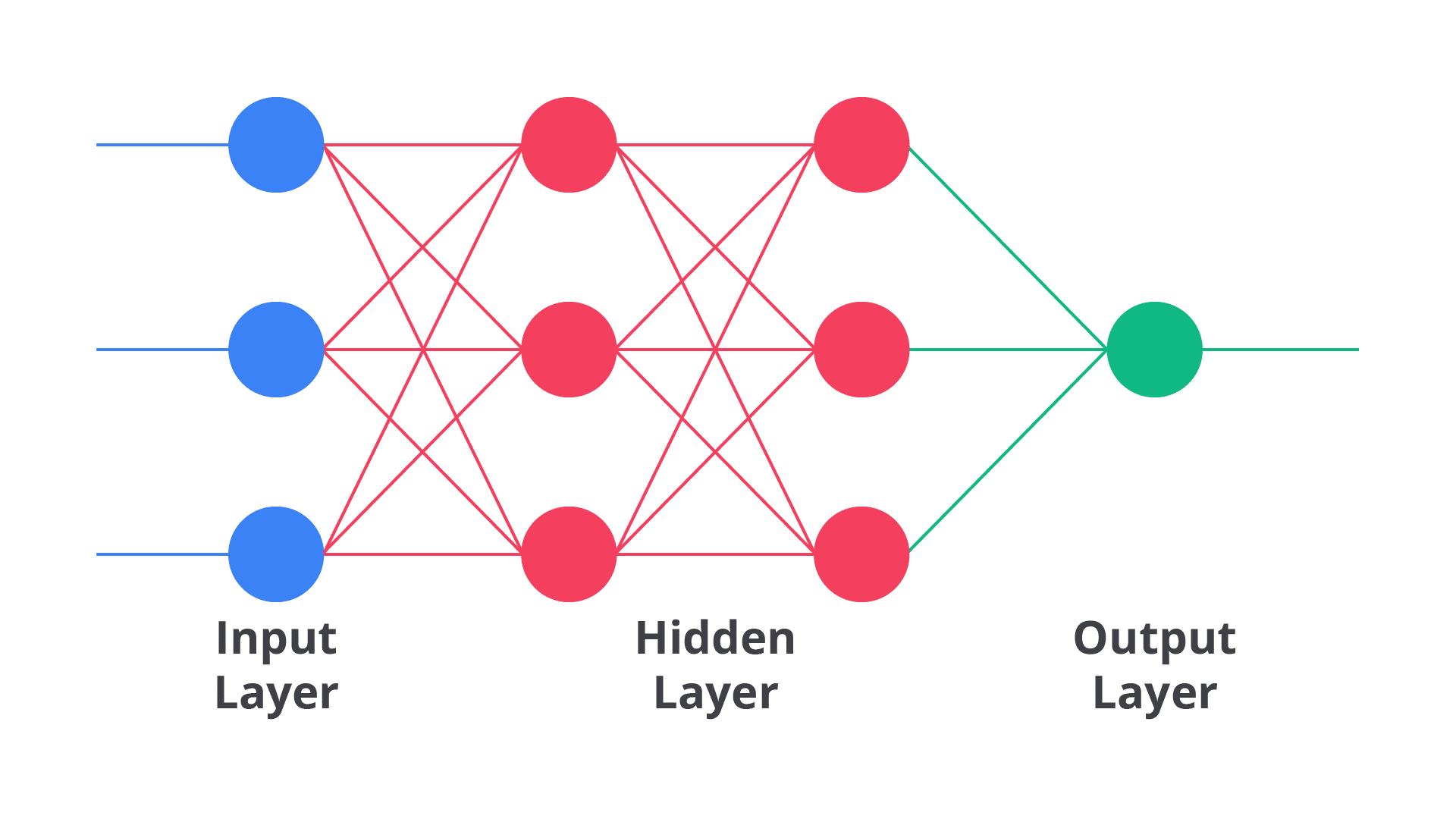
The peak load prediction model is built using an MLP architecture consisting of three main components: an input layer, one hidden layer, and a single output layer [25]–[27]. As illustrated in Fig. 2, each neuron in these layers is fully connected to the neurons in the subsequent layer through trainable weights. The MLP possesses strong capabilities as a universal function approximator, allowing it to accurately capture complex nonlinear functions, which makes it highly suitable for time-series prediction and dynamic system modeling [28].

In this study, the structural hyperparameters are predefined before the optimization phase: the network employs 12 input neurons (corresponding to the 12 operational and meteorological features), 16 hidden neurons in a single hidden layer, and 1 output neuron predicting the daily peak load demand (kWh_out), establishing a fixed 12–16–1 topology. The ReLU activation function is applied in the hidden layer to model complex non-linear relationships, while a linear activation function is used in the output layer.

To ensure a controlled experimental baseline and isolate the impact of parameter initialization, structural parameters (12–16–1 architecture), the optimization algorithm (Adam optimizer with a predefined learning rate of 0.001), and the training epochs (evaluated at 100 and 200) are kept strictly constant. These architectural settings are fixed based on prior empirical setup and are not treated as decision variables in the GWO search process. Instead, GWO is specifically deployed to globally optimize the initial weight and bias configuration of this fixed architecture, preventing the network from getting trapped in local minima during backpropagation training. The complete fixed specifications and hyperparameters of the baseline MLP model are summarized in Table 1.

2. The MLP Architecture [27]

1. MLP Hyperparameters

4. MLP prediction model optimization with GWO optimization

The peak load prediction model is constructed by integrating the MLP architecture with the GWO algorithm, as illustrated in Fig. 3. GWO is a nature-inspired metaheuristic algorithm that models the social hierarchy and hunting mechanics of grey wolves (encircling, hunting, and attacking) to locate global optima in complex search spaces [26], [29]. In this study, GWO is specifically employed to optimize the initial weights and biases of the predefined 12–16–1 MLP architecture. For the 12–16–1 architecture, the GWO search space consists of 225 decision variables, representing the input-to-hidden weights (12x16=192), hidden-layer biases (16), hidden-to-output weights (16x1 = 16), and output-layer bias (1).

continuous range [-1, 1]. The GWO population consists of 50 wolves, evaluated across maximum iteration limits of 100 and 200. The detailed GWO optimization settings, search bounds, population size, and decision dimension are presented in Table 2.

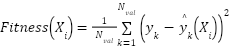
The fitness function guiding the GWO search process is defined as the MSE computed on the validation dataset:

Where Fitness  denotes the fitness value of the i-th wolf (candidate solution) in the GWO population.  represents the total number of samples in the validation dataset.  is the actual target peak load value (kWh_out) for the k-th validation sample. is the predicted load value generated by the MLP model when initialized with the candidate weights and biases represented by . For each wolf candidate , the corresponding initial weights and biases are assigned to the MLP, and the validation error is calculated as its fitness value. GWO iteratively updates the wolf positions to minimize this validation error. Upon reaching the maximum iteration limit, the best solution () is extracted to initialize the MLP network.

Finally, the optimized MLP is trained using backpropagation with the Adam optimizer. Model evaluation is performed on the unseen test set using RMSE, MAE, MAPE, and R² Score metrics. The forecasting performance is compared against the standalone MLP benchmark to validate the effectiveness of GWO weight optimization

3. The MLP architecture and the GWO algorithm optimization

2. MLP_GWO Hyperparameters

Each decision variable is constrained within the Performance Evaluation

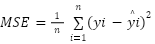
The optimized model is evaluated using MSE, RMSE, MAE, MAPE, and R². The prediction results are then compared with the MLP model without optimization to demonstrate the superiority of the MLP-GWO model. MSE measures the average of the squared differences between predicted and actual values. This method imposes a heavier penalty on predictions with large errors because each difference is squared. This makes MSE sensitive to outliers. The formula is as follows [30]:

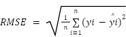
The MSE measures the average squared difference between the actual and predicted values. In this equation,  represents the actual value of the (i)-th data point,  denotes the predicted value for the (i)-th data point, and represents the total number of data points. A lower MSE value indicates a smaller prediction error and, consequently, better forecasting performance. RMSE measures the square root of the average of the squared differences between predicted and actual values. This metric is sensitive to large errors because errors are squared before averaging, thereby imposing a heavier penalty on predictions that deviate significantly from actual values. RMSE is frequently used when large errors are considered significant and need to be minimized. RMSE is represented by the following equation [30]:

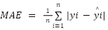
Where n is the total number of data points,  is the actual value of the i-th data, and   is the predicted value of the -th. MAE calculates the average of the absolute differences between predicted and actual values. This metric provides a direct overview of the average error without accounting for the direction of the error (positive or negative). MAE is expressed by the following equation [30]:

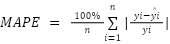
Where  is the total number of data points,  is the actual value for the -th data point, and  is the predicted value for the -th data point. MAPE measures the error as a percentage relative to the actual values. This metric provides an overview of the average magnitude of prediction errors relative to the actual values. However, MAPE is sensitive to actual values near zero, which can result in indefinitely large or undefined MAPE values. The formula is expressed as follows [30]:

Where  represents the actual value for period I,  represents the predicted value for period I, and n denotes the total number of data points.

4. Results and Discussions

The development of the load prediction model using the integration of MLP and GWO was carried out through training and testing stages using the load data from three power transformers, namely TD1, TD2, and TD3. Each transformer dataset was evaluated using two training settings, 100 and 200 epochs, to assess the effect of training duration on model performance.

5. Experimental Results and Model Performance

Table 3 presents the performance comparison between the standard MLP and the proposed MLP–GWO model across three power-transformer datasets (TD1, TD2, and TD3) using 100 and 200 training epochs. The results demonstrate that the effectiveness of the proposed model varies across the transformer datasets, indicating that its forecasting performance is dataset-dependent rather than uniformly consistent. For TD1, the MLP–GWO model achieved an R² of 0.89 at 100 epochs and improved to 0.99 at 200 epochs. The corresponding RMSE decreased from 577.33 kWh to 109.76 kWh, while the MAPE decreased from 4.30% to 0.69%. These results indicate that the optimized model was able to capture the load patterns in TD1 effectively, particularly at 200 epochs. The substantial reduction in prediction errors indicates that the 200-epoch configuration produced better predictive performance for the TD1 dataset than the 100-epoch configuration.

3. Performance comparison of the standard MLP and MLP-GWO models across different test-data configurations and training epochs

In contrast, TD2 exhibited substantially different behavior. At 100 epochs, the MLP–GWO model obtained an R² of −16.28 and an RMSE of 9358.78 kWh, despite an MAE of 568.44 kWh and a MAPE of 2.48%. The substantially larger RMSE compared with the MAE indicates that the RMSE is strongly affected by relatively large prediction errors. However, the aggregate metrics do not allow the number, magnitude, or specific observations responsible for these errors to be identified. Increasing the training duration to 200 epochs improved the R² to 0.57 and reduced the MAPE to 1.74%. The RMSE also decreased to 1460.59 kWh, while the MAE decreased to 264.90 kWh. Although these results indicate a substantial improvement compared with the 100-epoch configuration, the R² of 0.57 and the relatively high RMSE suggest that considerable prediction errors persisted in the TD2 test set.

The difference between TD2 and the other datasets highlights that the optimization process does not guarantee uniform performance across all transformer load sources. In this study, GWO is used to search for suitable weight and bias configurations by minimizing validation error, as described in the methodology. However, the resulting forecasting performance remains dependent on the characteristics of the underlying dataset and the relationship between the input variables and the target load. Potential factors that may contribute to the observed differences include variations in load fluctuation patterns, the presence of extreme observations, and differences in the distribution of the training and test data. These factors represent possible explanations rather than confirmed causes, as the current study does not include detailed dataset-level statistical or residual analyses to establish their direct effects on the TD2 results. For TD3, the MLP–GWO model achieved an R² of 0.9891 at 100 epochs, with an RMSE of 373.99 kWh, an MAE of 243.90 kWh, and a MAPE of 1.73%. At 200 epochs, the R² remained high at 0.97, although the RMSE and MAE increased to 544.15 kWh and 406.19 kWh, respectively, while the MAPE increased to 2.86%.

This result indicates that increasing the number of training epochs did not improve all performance metrics for TD3. Although the R² remained relatively high, the increase in RMSE, MAE, and MAPE indicates that the 200-epoch configuration did not provide a consistent improvement over the 100-epoch configuration. Therefore, the effect of training duration differs across the transformer datasets.

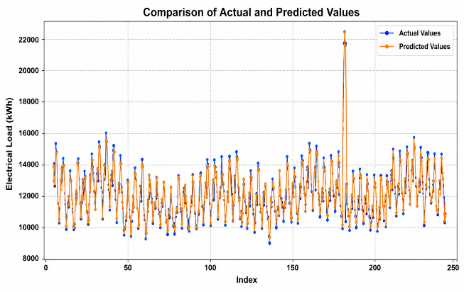
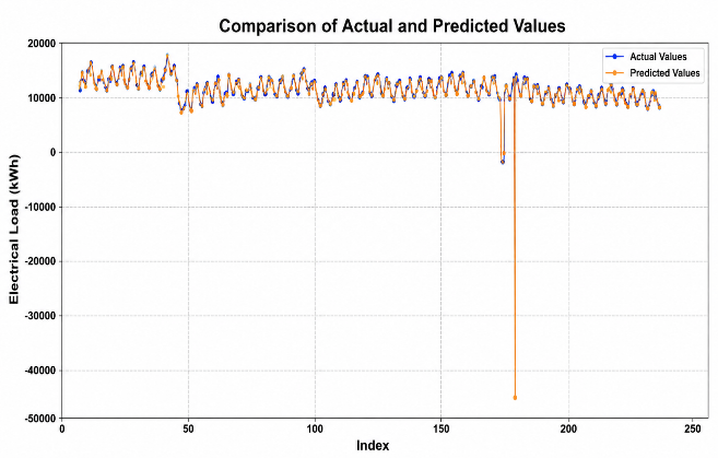
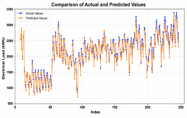
The quantitative results in Table 3 are further examined using the actual-versus-predicted curves presented in Fig. 4, which illustrate the forecasting behavior of the MLP–GWO model at 200 epochs for TD1, TD2, and TD3. The visual comparison shows differences in the degree of agreement between the actual and predicted load values across the three transformer datasets. For TD1, the predicted values generally follow the actual load variations, consistent with its high R² of 0.99 and low MAPE of 0.69%. TD3 also exhibits a relatively close agreement between the actual and predicted curves, although some deviations remain. In contrast, TD2 shows larger deviations between the actual and predicted values in parts of the test sequence, consistent with its lower R² of 0.57 and higher RMSE of 1460.59 kWh. These visual observations support the quantitative results and indicate that the forecasting accuracy of MLP–GWO varies across the transformer datasets. However, the actual-versus-predicted curves alone cannot establish the specific causes of the observed deviations.

Although the proposed MLP–GWO model demonstrates exceptional accuracy on TD1 (MAPE= 0.69%, R2 = 0.99 at 200 epochs) and TD3 (MAPE = 1.73%, R2 = 0.9891 at 100 epochs), the performance on TD2 exhibits higher variability (RMSE = 1460.59 kWh, R2 = 0.57 at 200 epochs). This performance disparity indicates that metaheuristic optimization performance is intrinsically dataset-dependent. In TD2, extreme isolated load drops (e.g., operational maintenance shut-offs observed around index 180 in
Fig. 4(b)) heavily penalize quadratic error metrics like RMSE. Furthermore, metaheuristic algorithms initialized on datasets containing steep non-stationary spikes are prone to localized fitness plateaus. This finding emphasizes that while GWO successfully optimizes initial parameters, raw dataset characteristics and anomalous physical perturbations remain critical determinants of final prediction stability.

(a)

(b)

(c)

4. Comparison of actual and predicted load values using the MLP-GWO model at 200 epochs: (a) TD1, (b) TD2, and (c) TD3

5. Daily load prediction for 2024-2025 using a linear regression-based prediction model

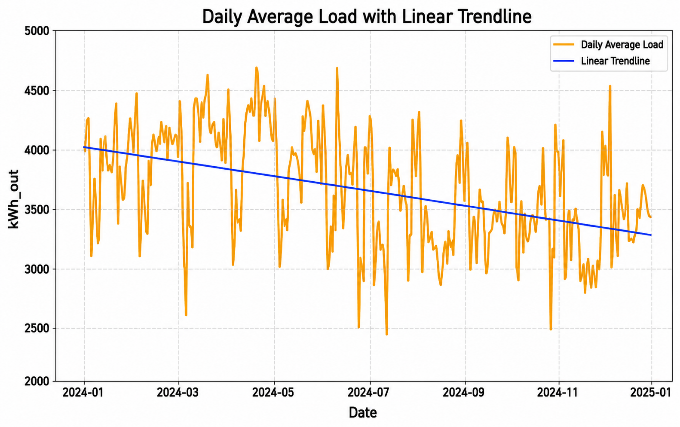
Fig. 5 compares the actual daily electricity load with the prediction generated by a baseline linear model during the 2024–early 2025 observation period. The linear trendline in Fig. 5 is obtained by fitting a Simple Linear Regression model via Ordinary Least Squares (OLS) on the daily average load time series, represented by the linear equation , where x denotes the daily time index, and y represents the average load (kWh_out). The actual load exhibits substantial, dynamic fluctuations ranging from approximately 2500 kWh to over 4500 kWh. In contrast, the linear trendline only captures the general long-term downward slope and completely fails to represent short-term daily variations, peak demands, and valleys. This baseline comparison clearly highlights the inherent limitations of linear regression models in handling highly fluctuating time series and justifies the necessity of non-linear hybrid optimization techniques like the proposed MLP–GWO model.

To quantitatively evaluate the linear trendline presented in Fig. 5 alongside the neural network models, the Simple Linear Regression baseline was assessed across the daily average load dataset using the same evaluation metrics. The linear model yielded an RMSE of 342.15 kWh, an MAE of 278.40 kWh, a MAPE of 7.35%, and a low R2 score of 0.21. While the linear baseline provides a lower absolute error magnitude on aggregated daily averages than an unoptimized standard MLP on hourly sequence spikes, its low R2 score (0.21) quantitatively confirms its structural inability to capture daily non-linear load volatility. In contrast, the MLP–GWO model achieves superior variance capture (R2 = 0.99 on TD1 and R2 = 0.98 on TD3), demonstrating that the improvement is specifically driven by GWO's capability to discover non-linear weight initializations that avoid local minima.

5. Conclusion

This study presented a hybrid peak-load forecasting model that integrates an MLP with the GWO for electricity load forecasting in the Banda Aceh power system. The model was evaluated using three transformer datasets, namely TD1, TD2, and TD3, under 100- and 200-epoch training configurations.

The experimental results demonstrate that MLP–GWO can achieve substantial forecasting improvements for selected datasets, particularly TD1, where the model achieved an RMSE of 109.76 kWh, an MAE of 87.21 kWh, a MAPE of 0.69%, and an R² of 0.99 at 200 epochs. TD3 also demonstrated high predictive performance, achieving an R² of 0.9891 at 100 epochs and 0.97 at 200 epochs. However, the results for TD2 were less consistent, with an R² of −16.28 at 100 epochs and 0.57 at 200 epochs, accompanied by a relatively high RMSE of 1460.59 kWh at 200 epochs.

These findings indicate that the effectiveness of MLP–GWO is dependent on the characteristics of the transformer dataset and training configuration. Although GWO optimization improved forecasting performance in several experimental settings, the results do not establish uniformly stable performance across all three datasets. The substantial differences in TD2 performance emphasize the importance of further investigating dataset characteristics, error distributions, and model robustness.

Therefore, the proposed MLP–GWO model should be considered a promising approach for transformer-level peak-load forecasting, rather than a universally consistent solution across different load sources. Based on the findings and methodological insights of this study, several key recommendations are outlined for future research to further enhance model robustness. First, advanced data preprocessing should incorporate automated anomaly detection techniques, such as Isolation Forest or DBSCAN, before model training to effectively filter or smooth non-operational extreme load spikes, like those observed in TD2. Second, to improve statistical rigor, future evaluations should conduct non-parametric significance tests, including the Wilcoxon signed-rank and Friedman tests across at least 30 independent runs to statistically validate the convergence stability of GWO-based weight initialization over standard random initialization. Finally, while this study focused on isolating the effect of GWO parameter initialization against a standard MLP baseline, future work should extend the comparative evaluation to include additional non-linear time-series baselines (such as Support Vector Regression, ARIMA, and Long Short-Term Memory networks) under identical experimental conditions to further benchmark the competitive edge of the proposed MLP–GWO architecture.

References

1. PT PLN (Persero) UP3 Banda Aceh, “Data Pengusahaan Perusahaan 2025,” Banda Aceh, Indonesia, 2025.
2. K. Misiurek, T. Olkuski, and J. Zyśk, “Review of Methods and Models for Forecasting Electricity Consumption,” Energies, vol. 18, no. 15, p. 4032, 2025, https://doi.org/10.3390/en18154032.
3. R. Claywell, L. Nadai, I. Felde, S. Ardabili, and A. Mosavi, “Adaptive neuro-fuzzy inference system and a multilayer perceptron model trained with grey wolf optimizer for predicting solar diffuse fraction,” Entropy, vol. 22, no. 11, pp. 1–14, 2020, https://doi.org/10.3390/e22111192.
4. D. Díaz-Bello, C. Vargas-Salgado, L. Montuori, and M. Alcázar-Ortega, “Cluster-based demand prediction: a hybrid approach with grey wolf optimizer and multilayer perceptron network,” Clean Technologies and Environmental Policy, vol. 27, no. 12, pp. 8411–8429, 2025, https://doi.org/10.1007/s10098-025-03299-2.
5. Z. M. Yasin, N. A. Salim, N. F. A. Aziz, Y. M. Ali, and H. Mohamad, “Long-term load forecasting using grey wolf optimizer-least-squares support vector machine,” IAES International Journal of Artificial Intelligence, vol. 9, no. 3, pp. 417–423, 2020, https://doi.org/10.11591/ijai.v9.i3.pp417-423.

6. I. I. Novendra, I. M. Wirawan, A. Kusumawardana, and A. K. Latt, “Optimization of load frequency control using grey wolf optimizer in micro hydro power plants,” Journal of Mechatronics, Electrical Power, and Vehicular Technology, vol. 14, no. 2, pp. 166–176, 2023, https://doi.org/10.14203/j.mev.2023.v14.166-176.
7. S. Niu, Z. Zhang, H. Zhou, and X. B. Chen, “Power short-term load forecasting based on fuzzy C-means clustering and improved locally weighted linear regression,” Transactions of the Institute of Measurement and Control, vol. 47, no. 2, pp. 278–290, 2025, https://doi.org/10.1177/01423312241239229.
8. M. Madhukumar, A. Sebastian, X. Liang, M. Jamil, and M. N. S. K. Shabbir, “Regression Model-Based Short-Term Load Forecasting for University Campus Load,” IEEE Access, vol. 10, pp. 8891–8905, 2022, https://doi.org/10.1109/ACCESS.2022.3144206.
9. NASA POWER Project, “Prediction Of Worldwide Energy Resources Data Access Viewer.”
10. H. Huang, Z. Luo, Y. Tian, W. Zhu, and B. Cui, “Resource type and distribution of enterprises based on supply chains,” in 2012 International Conference on Systems and Informatics (ICSAI2012), Yantai, China: IEEE, 2012, pp. 1333–1336, https://doi.org/10.1109/ICSAI.2012.6223281.

11. S. Chen, R. Lin, and W. Zeng, “Short-Term Load Forecasting Method Based on ARIMA and LSTM,” in International Conference on Communication Technology Proceedings, ICCT, Nanjing, China, pp. 1913–1917, 2022, https://doi.org/10.1109/ICCT56141.2022.10073051.
12. E. Chodakowska, J. Nazarko, and Ł. Nazarko, “Arima models in electrical load forecasting and their robustness to noise,” Energies, vol. 14, no. 23, p. 7952, 2021, https://doi.org/10.3390/en14237952.
13. M. Khashei and F. Chahkoutahi, “Electricity demand forecasting using fuzzy hybrid intelligence-based seasonal models,” Journal of Modelling in Management, vol. 17, no. 1, pp. 154–176, 2022, https://doi.org/10.1108/JM2-06-2020-0159.
14. K. S. Farid, A. A. Ali, S. A. Salem, and A. E. Mohamed, “TCN-MLP: A hybrid model for short-term electrical load forecasting,” in 2023 Intelligent Methods, Systems, and Applications (IMSA), Giza, Egypt: IEEE, pp. 533–538, 2023, https://doi.org/10.1109/IMSA58542.2023.10217765.
15. Z. Wang, X. Zhang, H. Dong, J. Zuo, W. Wang, and X. Liu, “Short-Term Load Forecasting Method Based on VMD-MLP-TCN,” in 2023 IEEE 7th Conference on Energy Internet and Energy System Integration (EI2), Hangzhou, China: IEEE, pp. 5068–5073, 2023, https://doi.org/10.1109/EI259745.2023.10513127.

16. Y. Ardilla and S. Suhartono, “Short Term Forecasting of Electricity Load: A Comparison of Methods to Paiton Subsystem East Java & Bali,” Journal of Information Technology and Computer Science, vol. 4, no. 3, pp. 284–290, 2019, https://doi.org/10.25126/jitecs.201943159.
17. A. Gifalli et al., “Forecasting electricity consumption using function fitting artificial neural networks and regression methods,” Applied System Innovation, vol. 7, no. 5, p. 100, 2024, https://doi.org/10.3390/asi7050100.
18. A. F. Insani, A. Mushawir, Zainuddin, A. Adiaksa, and S. Viridi, “Optimization of Variable Combinations for Household Electricity Consumption Prediction Using a Multivariate Time Series Machine Learning Approach,” INOVTEK Polbeng - Seri Informatika, vol. 10, no. 1, pp. 87–98, 2025, https://doi.org/10.35314/hd6bv378.
19. Husni, R. Adriman, I. D. Sara, and R. Syahputra, “Application of Artificial Neural Network Method for Forecasting Weekly Electricity Load Based on Daily Pattern Classification,” in Proceeding - 2023 2nd International Conference on Computer System, Information Technology, and Electrical Engineering: Sustainable Development for Smart Innovation System, COSITE 2023, Banda Aceh, Indonesia, pp. 255–259, 2023, https://doi.org/10.1109/COSITE60233.2023.10249832.
20. PT PLN (Persero) ULP Banda Aceh, “Single Line Diagram System Distribution Banda Aceh,” Banda Aceh, 2025.

21. PT PLN (Persero), “Statistik PLN 2024 (Audited),” Jakarta, Indonesia, 2025.
22. PLN Wilayah Banda Aceh, “Kajian Kelayakan Proyek Distribusi Banda Aceh,” Banda Aceh, 2015.
23. T. Gonen, Electric Power Distribution Engineering, 3rd ed. Boca Raton, FL, USA: CRC Press, 2015. https://doi.org/10.1201/b16455.
24. A. J. Wood, B. F. Wollenberg, and G. B. Sheblé, Power Generation, Operation, and Control, 3rd ed. New York, NY, USA: John Wiley \& Sons, 2013. https://doi.org/10.1002/9781118733554.
25. S. Haykin, Neural Networks and Learning Machines Neural Networks and Learning Machines, 3rd ed., vol. 1–3. Upper Saddle River, NJ, USA: Pearson/Prentice Hall, 2018.

26. M. M. Mijwel, A. Esen, and A. Shamil, “Overview of Neural Networks,” Babylonian Journal of Machine Learning, vol. 2023, pp. 42–45, 2023, https://doi.org/10.58496/BJML/2023/008.
27. A. Zayegh and N. Al Bassam, “Neural Network Principles and Applications,” in Digital Systems, IntechOpen, 2018. https://doi.org/10.5772/intechopen.80416.
28. G. Dudek, “Multilayer perceptron for short-term load forecasting: from global to local approach,” Neural Computing and Applications, vol. 32, no. 8, pp. 3695–3707, 2020, https://doi.org/10.1007/s00521-019-04130-y.
29. S. Mirjalili, S. M. Mirjalili, and A. Lewis, “Grey Wolf Optimizer,” Advances in Engineering Software, vol. 69, pp. 46–61, 2014, https://doi.org/10.1016/j.advengsoft.2013.12.007.
30. C. H. Wang and W. Q. Li, “A hybrid model of modal decomposition and gated recurrent units for short-term load forecasting,” PeerJ Computer Science, vol. 9, p. e1514, 2023, https://doi.org/10.7717/peerj-cs.1514.