Comparative Analysis of PI Anti-Windup and Adaptive Fuzzy PID for Output Voltage Control of a Non-Inverting Buck-Boost DC-DC Converter

Sofyan Muhammad Ilman 1,*, Febi Ariefka Septian Putra 2, Rafly Heriansyah 3, Toha Rohimat 4, Toto Tohir 5,
Giga Verian Pratama 6, Muhammad Nuruddin Ar-Rabbani 7

1, 2, 3, 4, 5, 6 Department of Electrical Engineering, Politeknik Negeri Bandung, Bandung, Indonesia

7 Department of Electrical Engineering, Faculty of Engineering, Tanjungpura University, Pontianak City, Indonesia

Email: 1 sofyan.muhammad@polban.ac.id, 2 febi.ariefka@polban.ac.id,
3 rafly.heriansyah.toi22@polban.ac.id, 4 toha.rohimat.toi22@polban.ac.id, 5toto.tohir@polban.ac.id,
6 giga.verian@polban.ac.id, 7 nuruddin.ar@ee.untan.ac.id

*Corresponding Author

Abstract—Buck-Boost Non-Inverting DC-DC converters are widely used in DC power supply and battery-based systems because they can raise or lower the output voltage without reversing the output polarity. However, the converter's nonlinear characteristics make voltage control more complex, especially when the load or set point changes. This study compares the performance of two voltage control strategies, namely Proportional-Integral Anti-Windup (PI-AW) and Adaptive Fuzzy PID (AFPID), on DC-DC Buck-Boost Non-Inverting converters. The system is designed to operate in buck mode with an output voltage of 12 V and boost mode with an output voltage of 24 V from a 15 V input voltage source, using a load variation of 100–300 Ω and a switching frequency of 30 kHz. Evaluation was carried out through PSIM simulation and ESP32-based hardware implementation, with test scenarios including fixed set points, set-point changes, and load changes. The test results showed that both methods adjusted the output voltage to follow the reference value under all test conditions. However, the Anti-Windup PI performed better than the Adaptive Fuzzy PID, with faster rise times, lower overshoot and steady-state errors, shorter settling times, and smaller voltage ripples in buck and boost modes. The results show that PI Anti-Windup is more suitable for DC-DC Buck-Boost Non-Inverting converters that require fast transient response and high output-voltage stability.

Keywords—Adaptive Fuzzy PID; Anti-Windup PI; Buck-Boost Non-Inverting; Dynamic Response; Voltage Control

1. Introduction

Advances in power converter technology are growing rapidly, particularly in DC power supply system applications and battery-based systems, which require stable output voltage despite changes in load or input voltage [1]. Modern applications such as battery charging systems, Battery Management Systems, solar power plants (photovoltaic), and voltage stabilizers in portable picohydro renewable energy systems rely heavily on DC-DC converters to regulate output voltage constantly and precisely [2].

One of the most widely used topologies is the DC-DC Buck-Boost Non-Inverting converter because it can raise or lower the voltage without changing the output polarity [3]. Researchers have also pursued various transformerless topologies with continuous input current and positively polarized outputs to increase voltage gain and expand conversion ratios. This capability makes it a strong choice for portable devices, LED drivers, battery management systems, and renewable energy systems with a wide operating voltage range [4]. However, because the two active switches are controlled separately in buck and boost operating modes, the converter exhibits highly nonlinear and complex dynamics, particularly during mode transitions [5].

Converter performance is strongly dependent on the control strategy, and conventional voltage control in four-switch buck–boost converters still show dynamic-response limitations, especially overshoot and long settling time under wide operating conditions and disturbances [6]. One reference study reported a recovery time of 0.1 to 0.5 seconds with an overshoot of 22.93%. In addition, conventional Proportional-Integral (PI) controllers can experience integrator windup [7]. Excessive accumulation in the integral part when the actuator is saturated, which causes saturation of the control signal and slows down the transient response [8].

To address these limitations, researchers developed various control strategies. This research focuses on two approaches: Proportional-Integral Anti-Windup and Adaptive Fuzzy PID. The Anti-Windup PI approach adds a back-calculation mechanism to limit integral accumulation when the control signal saturates, keeping the transient response fast without overshooting [9]. Among the available control methods, the Adaptive Fuzzy PID Controller (AFPID) has received significant attention because it combines conventional PID control with the flexibility of fuzzy logic [10]. Fuzzy PID with a self-tuning mechanism can improve system control performance compared to classic PID.

Transient analysis results show that Fuzzy PID provides better robustness, improves step-response quality, and reduces response time. With its adaptive architecture, Fuzzy PID also provides a wide range of adjustments to setpoint changes and interference, making it more suitable for both nonlinear and dynamic system applications [11]. Artificial neural networks can also serve as an alternative to fuzzy logic systems, so this approach remains relevant for artificial intelligence-based control designs. Previous studies have developed both methods separately and tested DC-DC Buck-Boost Non-Inverting converters with the same specifications [12]. However, no studies have compared their performance in an equivalent testing framework. Therefore, this study aims to analyze and compare the performance of PI Anti-Windup and Adaptive Fuzzy PID control on DC-DC Buck-Boost Non-Inverting converters, using rise time, settling time, overshoot, and steady-state error as the main indicators under fixed setpoint conditions, setpoint changes, and load changes.

The objectives of this research are as follows. First, design and implement two voltage control systems, namely PI Anti-Windup and Adaptive Fuzzy PID, on DC-DC Buck-Boost Non-Inverting converters with identical specifications. Second, test both systems' performance through PSIM simulation and ESP32-based hardware implementation. Third, compare the two methods based on rise time, settling time, overshoot, steady-state error, and voltage ripple across various operating scenarios.

This study directly compares the anti-windup-based control approach and the fuzzy-based adaptive control approach on the same converter platform. This comparison is important as a basis for choosing a control strategy that suits the application's needs, emphasizing response speed, stability, and adaptability to changing operating conditions.

2. Proposed and Research

1. DC-DC Buck-Boost Non-Inverting Converter

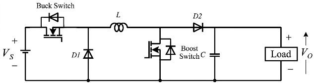
A buck-boost converter is a DC-DC converter used to increase or decrease voltage. In the ideal buck-boost (IBB) circuit, only one semiconductor switch, such as a MOSFET, IGBT, or transistor, is usually used. The array looks simple, but it has a basic drawback: the output voltage has inverted polarity relative to the source [13].

To address this issue, a series of Non-Inverting Buck-boost Converters (NIBBC) was developed. In this topology, one switch is added so the output voltage has the same polarity as the input voltage. Conceptually, the Non-Inverting Buck-Boost Converter combines a buck converter and a boost converter, with a MOSFET switch that operates according to its mode [13].

When the input voltage exceeds the output voltage, the converter operates in buck mode. In this mode, one MOSFET is activated to lower the voltage while storing energy in the inductor, and then that energy is delivered to the load through the diode when the MOSFETs are idle. Conversely, when the input voltage is lower than the output voltage, the system switches to boost mode. In this mode, the first MOSFET charges the inductor, and when it turns off, the second MOSFET activates to deliver that energy to the load, increasing the output voltage [14].

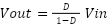
In Fig. 1, the ideal DC-DC converter: the relationship between the output voltage and the input voltage in this converter depends on the duty cycle (D) of the PWM signal. In buck mode, the output voltage is smaller than the input voltage, while in boost mode, the output voltage is greater than the input voltage, as stated in the (1) [15].

Vout is the output voltage, Vin is the input voltage, and D is the duty cycle, which is in the range 0 to 1. Because the converter's characteristics are nonlinear and depend on the operating point, a control strategy is needed to maintain output-voltage stability in both operating modes without excessive overshoot or oscillation.

1. Non-inverting buck-boost circuit

1. Anti-windup PI Control

The Proportional-Integral (PI) controller is widely used because it is simple and able to eliminate steady-state errors through integral action. However, when the control signal reaches the actuator saturation limit, the integral part continues to accumulate even though the output can no longer increase. This phenomenon, called integrator windup, causes large overshoot and a slow recovery response. The Anti-Windup mechanism, especially the back-calculation method, corrects the accumulation of excess integrals so the control signal quickly returns to the linear operating range [16].

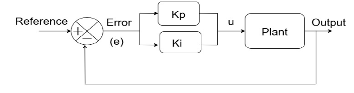
Fig. 2 illustrates the closed-loop control structure using a proportional-integral (PI) controller, where the control signal is generated from the error  between the reference and feedback signals. Mathematically, the PI controller output is given as follows,

where e(t) is the difference between the set point and the rated output voltage, Kp is the proportional gain, and Ki is the integral gain. In the back-calculation mechanism, the difference between the control signal before and after saturation is fed back to reduce the integral accumulation rate through the tracking time constant, so the integrator does not continue to accumulate when the duty cycle reaches the maximum or minimum limit. Thus, the transient response remains fast, and the overshoot can be suppressed even when the actuator is briefly saturated [17].

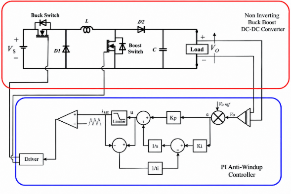
To overcome this problem, a PI controller with an Anti-windup mechanism was developed. In the Anti-Windup PI structure, the control signal resulting from the sum of proportional and integral actions is first passed through the saturation block to ensure the control signal does not exceed the physical limits of the actuator [18]. The difference between the control signal before and after saturation is then calculated and multiplied by an Anti-windup gain Ks, which is returned as feedback to the integrator. This mechanism corrects or limits integral accumulation while the actuator is saturated, preventing excessive error accumulation and minimizing integrator windup [19].

2. Schematic diagram of PI blocks

Fig. 3 is the circuit topology of the non-inverting buck-boost converter, consisting of a buck switch, boost switch, two diodes ( and ), an inductor , and an output capacitor . The converter is capable of operating in both buck and boost modes while maintaining a non-inverted output voltage polarity. To overcome windup, researchers have developed and implemented various anti-windup techniques, such as conditional integration, back-calculation, and saturating integrators. Experimental studies and simulations show that applying anti-windup techniques to PI controllers can significantly improve system performance, reduce overshoot, and speed up recovery time in both linear and nonlinear systems. Anti-windup is especially important in systems prone to actuator saturation, helping the system remain stable and responsive. The formula for the anti-windup PI with back calculation is as follows,

where represents the control signal generated by the PI controller, is the proportional gain, and  is the integral gain. The term denotes the control error, defined as the difference between the reference signal and the measured output. The variable represents the Laplace operator. The term denotes the integral time constant, which determines the dynamic response of the integral action. Meanwhile,  represents the saturated control signal, which is limited according to the allowable operating range of the converter. The difference forms the anti-windup back-calculation term, which prevents excessive accumulation in the integral component when the controller output reaches its saturation limit.

3. Design buck-boost non inverting converter PI-AW control

1. PI-AW tuning with the Ziegler-Nichols method 1

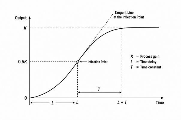
The control parameters are tuned using the Type I Ziegler-Nichols method. This process aims to obtain control parameters that produce a fast, stable system response with a low error rate. The Type I Ziegler-Nichols method is an empirical tuning method based on the system's response characteristics under open-loop conditions.

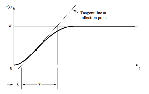
Fig. 4 is a first-order process reaction curve used for determining the process gain , dead time , and time constant . For this method, the plant provides an open-loop response curve. The next step is to determine the inflection point, the point with the largest change in gradient on the S-shaped curve. The tangent intersection results yield two main parameters: L as dead time and T as a time constant. These parameters then form the basis for determining the control parameters using the Type 1 Ziegler-Nichols tuning rule [20].

4. S response curve open loop system

With,

Table 1 shows the rule control parameters. The output voltage response curve was taken while testing the target duty cycle values of 44.44% and 61.54%. After that, calculations are carried out to obtain the PI -AW control parameters, and direct tests are carried out under PI-AW control.

1. Ziegler Nichols Rule Control Parameters 1

2. AFPID Control

Fuzzy logic in system modeling uses variables and linguistic propositions with a degree of truth between 0 and 1. The membership function converts real (crisp) input into a membership value and can be represented by various geometric curves, such as triangles, trapezoids, S, or Z [21]. This connection between qualitative representations is then formulated into the if–then rule base as the basis for decision-making and control actions [22].

A fuzzy inference system commands the data-processing mechanism that produces a crisp output. The process starts with fuzzifying the input signal, then selects rules using logical operators (AND, OR, NOT) and implication methods. The output of each rule is then combined in the aggregation stage, before finally being converted back into numerical form through a defuzzification process based on popular algorithms such as Tsukamoto, Mamdani, or Sugeno [23].

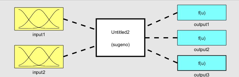
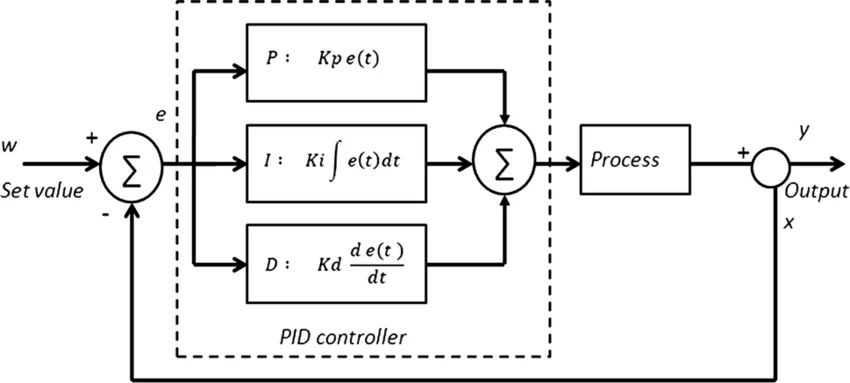
Fig. 5 schematically represents a Sugeno fuzzy inference system, showing two inputs processed to generate three output functions. The variable arrangement of processes in a system generally utilizes the Proportional-Integral-Derivative (PID) feedback control algorithm. This algorithm modifies the output signal by integrating three main control actions: proportional, integral, and derivative [24]. In the block diagram, the PID control system can be described as follows.

Fig. 6 is a block diagram of a conventional PID feedback control system, illustrating the proportional (P), integral (I), and derivative (D) control actions applied to the error signal to regulate the process output. Mathematically, the characteristics and responses of PID controllers are formulated through the following general equations:

5. Fuzzy Logic Controller's control structure

6. PID control block diagram

1. AFPID Tuning

Fuzzy sets are in charge of mapping human qualitative reasoning—which is full of uncertainty into mathematical form. There are three basic concepts in fuzzy logic: linguistic variables, fuzzy propositions, and membership functions. These three pillars integrate abstract descriptions into measurable mathematical models for control applications. Linguistic variables define a variable's value through phrases or words in natural language rather than numbers [25].

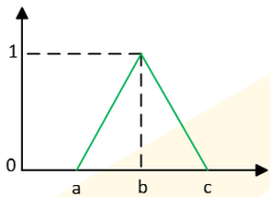
TS (Duty cycle) = {small, medium, big} = {S, M, B}, the function of a triangular membership is defined by three parameters, namely (a, b, c), which represent the starting limit, the peak point, and the end limit of the curve [26], as shown in Fig. 7.

Fig. 7 is a triangular membership function used in a fuzzy logic system, characterized by the parameters , , and , where represents the point of maximum membership (). The fuzzy inference process is carried out through a series of structured computational stages. The initial stage begins with input fuzzification, which maps the input crisp value to the membership degree of the predefined fuzzy set. Furthermore, fuzzy operators (such as AND, OR, and NOT) combine multiple antecedent conditions. This step is followed by an implication method that evaluates the if–then rule base to extract the output (sub-conclusion) of each active rule [27].

7. Triangle curve

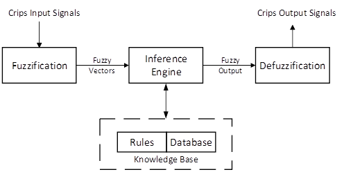
Fig. 8 shows a block diagram of a fuzzy inference system, illustrating fuzzification, fuzzy inference, and defuzzification, with the fuzzy rule base and knowledge base supporting the inference process. The output voltage regulation of the non-inverting buck-boost converter applies a combination of the Adaptive Fuzzy-PID (AFPID) scheme and the Type 1 (ZN1) Ziegler-Nichols tuning method. In this scheme, the initial PID constants (Kp, Ki, and Kd) are determined from the system's open-loop response curve using the time constant (T) and delay time (L) [28].

Furthermore, fuzzy logic adapts the ZN1 reference parameter in real time according to the system dynamics. This adjustment is based on two main inputs, namely voltage error (the difference between the set point and the voltage divider reading) and delta error (the rate of change in error). The AFPID controller then converts its output into a PWM signal to modulate the MOSFET gate switch [29].

8. Fuzzy inference system

Fig. 9 is a process reaction curve illustrating the determination of the process gain , dead time , and time constant  using the tangent-line method at the inflection point. The first-type Ziegler-Nichols method determines the controlling parameters using the empirical formulation listed in Table 2. The values of proportional constants (Kp), integral time (Ti), and derivative time (Td) are calculated directly using the two main variables of the S-shape response curve, namely delay time (L) and time constant (T). For full PID control, the gain magnitude is formulated as Kp = 1.2xT/L, with the integration time constant Ti = 2L and the differentiation time constant Td = 0.5L. This formulation produces responsive system responses while providing initial tuning parameters ready to be integrated or further adapted by intelligent algorithms such as fuzzy logic [30].

9. S-shape response curve

2. PID Parameter Formula

At the output design stage, the system uses the zero-order Sugeno fuzzy logic inference method. The PID parameter adjustment (auto-tuning) uses three output variables: proportional (dKp), integral (dKi), and derivative (dKd) gain changes. In contrast to input variables that use membership functions, the output in the zero-order Sugeno method is represented as a constant value (singleton or crisp value). Each output variable is divided into five linguistic parameters, namely Negative Big (NB), Negative Small (NS), Zero (Z), Positive Small (PS), and Positive Big (PB), which are symmetrically distributed in the range -1 to 1 [31]. The fuzzy logic rule base is arranged in a 5x5 matrix that correlates the error variable and delta error. This rule modulates the duty cycle adaptively, providing aggressive correction for large errors and smoothing the response around setpoints to reduce overshoot and maintain system stability [32].

3. Results and discussion

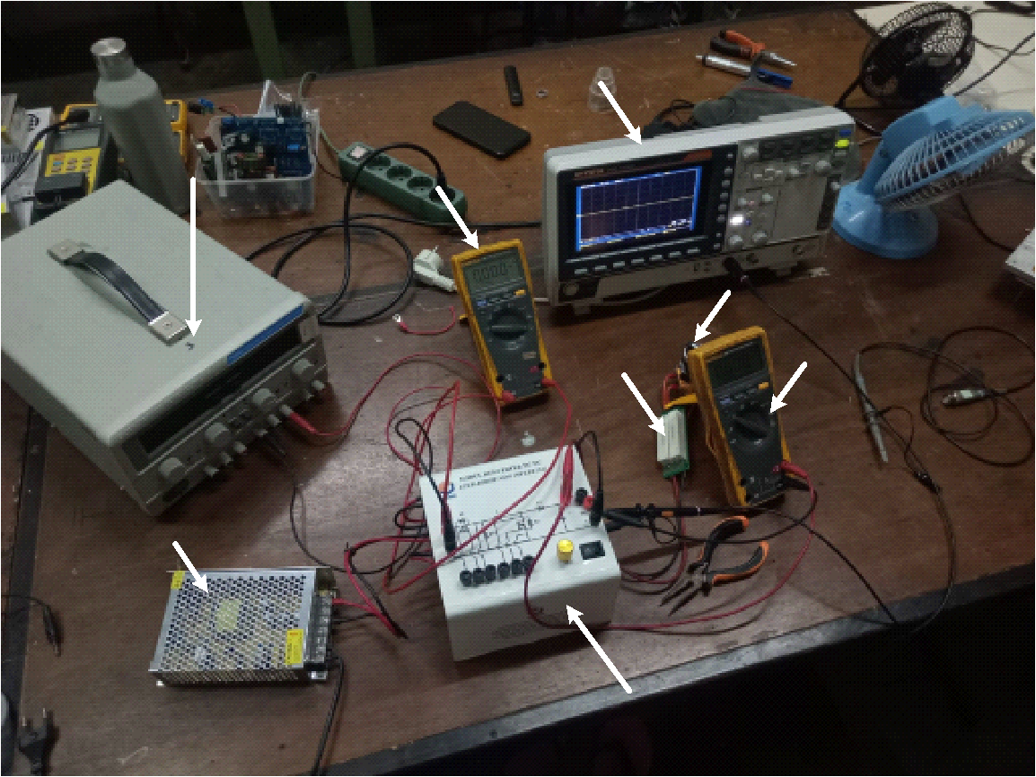
This research was carried out in two stages: simulation using PSIM software and experimental testing. In the simulation stage, we tested the system by changing the setpoint and introducing load-change interference to evaluate the controller's response. Furthermore, at the experimental stage, voltage control testing was carried out using PI control on the realized prototype. All designed hardware was then assembled into a single system so each component could function in an integrated manner, simplifying data retrieval and processing. Fig. 10 shows the overall hardware configuration used in this study.

10. Configuration of Non-Inverting Buck Boost Converter

The input voltage source in the Non-Inverting Buck-Boost Converter system is a 15 V DC power supply, which serves as the converter's main power supply. The control system uses an ESP32 microcontroller that gets power through the regulator module, while the gate driver circuit gets power as needed. The output voltage is measured with a voltmeter, while the input and output currents are measured with an ammeter. The test was carried out using resistive loads of 100 Ω and 300 Ω selected according to the test scenario. During the test, the oscilloscope was used to observe the output voltage response under fixed set-point conditions, set-point changes, and load changes to evaluate the performance of the PI-AW and AFPID control systems on the Non-Inverting Buck-Boost Converter.

Table 3 presents the specifications for the DC–DC non-inverting buck–boost converter, including input and output voltages, switching frequency, power rating, inductance, capacitance, load resistance, and diode and MOSFET ratings.

3. Specification of DC-DC Non-Inverting Buck Boost Converter

2. Determination of the PI-AW constant

To determine the PI-AW Constant, you need an S-curve graph to find the constant value for the buck and boost modes.

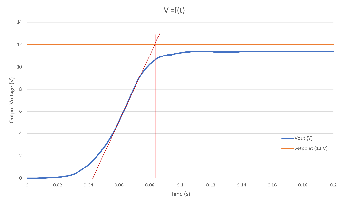
Fig. 11 shows the experimental output-voltage response of the DC–DC non-inverting buck–boost converter for a 12 V reference, illustrating the transient response, steady-state output voltage, and the tangent-line method used to determine the process parameters. From the graph of the output voltage open-loop response in buck mode, the value of the constant for each value of L = 0.044 and T = 0.05 is then substituted into the equation, thus producing the value of the PI-AW control parameter as in Table 4.

11. Buck mode open loop output voltage response picture

4. Buck mode PI-AW Control Parameters

Table 4 presents the PI-AW control parameters for the buck mode, including the proportional gain , integral time , and anti-windup gain . For the constant parameters of the boost mode, a line drawing is also carried out on the S-curve.

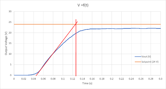
Fig. 12 shows the experimental output-voltage response of the DC–DC non-inverting buck–boost converter for a 24 V set point, illustrating the transient response and the steady-state output voltage, with the tangent-line method applied to determine the process parameters. From the graph of the output voltage open-loop response in boost mode, the value of the constant for each value of L = 0.042 and T = 0.078 is then substituted into the equation, thus producing the value of the PI-AW control parameter as in Table 5.

Table 5 presents the PI-AW control parameters for the boost mode of the DC–DC non-inverting buck–boost converter. The parameters consist of the proportional gain , integral time s, and anti-windup gain . These parameters regulate the converter output voltage in boost operation and improve the controller's dynamic response while limiting integrator windup during actuator saturation.

12. Open loop output voltage response picture boost mode

5. Control Parameters of PI-AW Boost Mode

3. PI-AW Testing

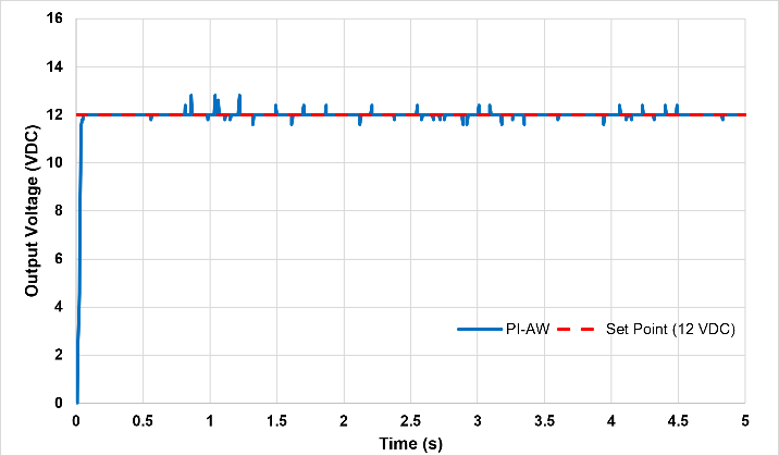
PI-AW control testing was performed on the Buck-Boost DC-DC Non-Inverting Converter using a load of 100 Ω. The results of the PI-AW control test in buck mode are shown in the following graph in Fig. 13.

13. Buck mode PI-AW control testing output voltage graph

Fig. 13 shows the experimental output-voltage response of the PI-AW controller for a 12 V set point, demonstrating the controller's ability to regulate the output voltage around the desired reference with small transient fluctuations. Based on the PI-AW control test results, the output voltage response shows fluctuations, with an overshoot of 13 VDC and an undershoot of 11.5 VDC. The analysis results for the output voltage response parameters are shown in Table 6.

6. Buck Mode PI-AW Control Test Response Parameters

Table 6 presents the experimental test-response parameters of the PI-AW controller in buck mode, including settling time, maximum peak, maximum undershoot, and steady-state error. Next, we test PI-AW control on the DC-DC converter in non-inverting buck-boost mode with a
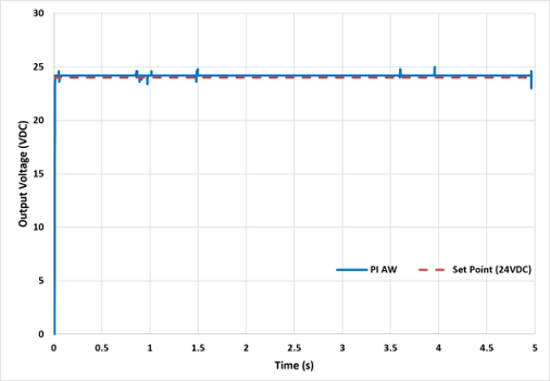
100 Ω load. The results of the PI-AW control test in boost mode are shown in the following graph in Fig. 14.

Fig. 14 shows the experimental output-voltage response of the PI-AW controller in boost mode for a 24 V set point. The response demonstrates that the controller rapidly regulates the converter output voltage around the reference value, with small transient fluctuations and a relatively small steady-state deviation. Based on the PI-AW control test results, the output voltage response shows fluctuations, with an overshoot of 24.5 VDC and an undershoot of 23 VDC. Table 7 shows the results of the output voltage response parameter analysis.

14. Output voltage graph testing PI-AW boost mode

7. PI-AW Control Test Response Parameters Boost Mode

Table 7 presents the experimental test-response parameters of the PI-AW controller in boost mode for the 24 V output-voltage reference. The table summarizes the main dynamic performance indicators, namely settling time, maximum peak, maximum undershoot, and steady-state error. The PI-AW controller achieves a settling time of 0.02 s, indicating that the output voltage reaches and remains within the specified settling band relatively quickly. The maximum peak is 4.2%, representing the highest overshoot of the output voltage relative to the 24 V reference during the transient response. Meanwhile, the maximum undershoot is 2.1%, indicating a small temporary deviation below the reference during the transient. Finally, the steady-state error is 0%, showing that the controller can regulate the output voltage to the desired 24 V reference under steady-state conditions.

4. Determination of AFPID constants

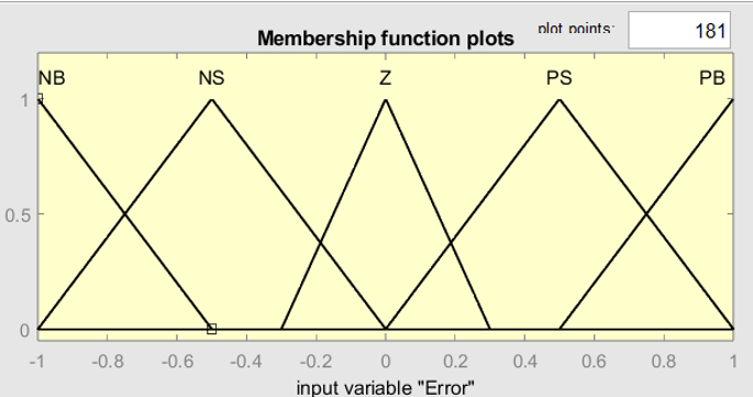
In the system design phase, the Error input variable is modeled using a triangular membership function distributed over the talk universe [-1, 1]. These variables are divided into five overlapping fuzzy sets: Negative Big (NB), Negative Small (NS), Zero (Z), Positive Small (PS), and Positive Big (PB). Each set has a center point placed symmetrically at -1, -0.5, 0, 0.5, and 1.

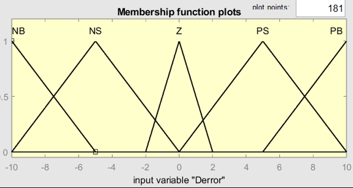
Fig. 15 and Fig. 16 present the membership functions of the error input in the fuzzy controller, consisting of five linguistic variables: NB, NS, Z, PS, and PB, with different input ranges for error scaling and fuzzy control processing. After determining the membership functions of the two inputs, a constant weight (singleton/crisp value) was determined for the zero-order Sugeno output variable (dKp, dKi, dKd) in the range [-1, 1]. Values are grouped symmetrically: NB (-1) and NS (-0.5) reduce PID gain, Z (0) maintains the reference parameters, and PS (0.5) and PB (1) increase gain when the response deviates.

Table 8 presents the output set constant parameters for the fuzzy controller, defining the incremental values of , , and  for each linguistic variable from NB to PB. Furthermore, we designed the fuzzy rules using a rule base and arranged the fuzzy logic in a 5×5 matrix that correlates the error variables and delta errors, as shown in Table 9.

15. Membership function error

16. Δerror membership functions

8. Output Set Constant Parameter Table

9. Fuzzy Rules Table

Table 9 presents the fuzzy rule base used in the fuzzy controller, which determines the appropriate control output based on the combination of the error and error-change linguistic variables. The rules use five linguistic categories, namely NB, NS, ZE, PS, and PB, to represent negative, zero, and positive conditions. These rules provide the basis for adjusting the controller parameters based on the magnitude and direction of the error, enabling the controller to improve the transient response and keep the output voltage close to its reference value. After successfully designing the fuzzy system, the PID control system is designed as the main control system.

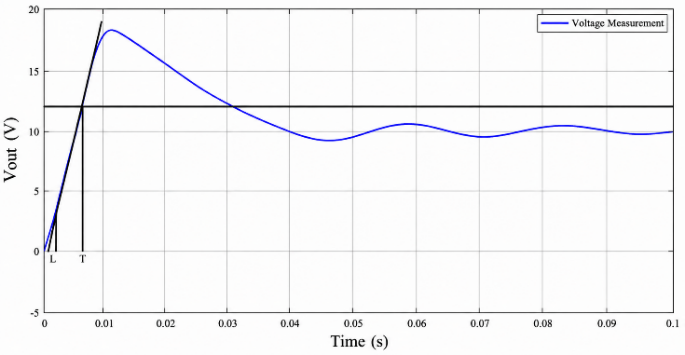
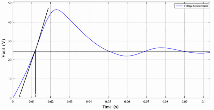
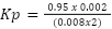
Fig. 17 and Fig. 18 show the open-loop test results of the DC–DC non-inverting buck–boost converter in Simulink/MATLAB for buck and boost operating modes, respectively. The response curves illustrate the output-voltage transient behavior, and the tangent line through the inflection point is used to determine the process parameters, particularly the dead time L and time constant T. These parameters then form the basis for calculating the controller gains. Table 10 presents the PID controller parameter calculations for buck mode based on the process parameters obtained from the open-loop response. The calculated parameters are the proportional gain Kp = 2.4, integral gain Ki = 600, and derivative gain Kd = 0.0024. These PID parameters provide the initial controller settings for regulating the converter output voltage in buck mode and serve as a reference for subsequent PI-AW controller tuning.

Table 11 presents the PID controller parameter calculation for the boost mode of the DC–DC non-inverting buck–boost converter. The controller parameters are obtained from the process characteristics identified through the open-loop response. Based on the calculation, the proportional gain is , the integral gain is , and the derivative gain is . These calculated gains are used as the initial PID tuning parameters for boost-mode operation and provide a basis for subsequent PI-AW controller implementation and performance evaluation.

17. Open-loop buck testing

18. Open-loop boost testing

10. Calculation Table of Buck Mode PID Parameters

11. Calculation Table of Boost Mode PID Parameters

5. AFPID Testing

After designing the system, tests are conducted to evaluate the response from the AFPID that has been developed.

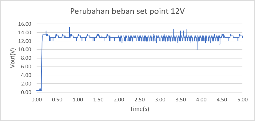
Fig. 19 presents the experimental output-voltage response under load variation at a 12 V set point, showing that the output remains regulated around the reference value despite load changes. The 5-second test result graph shows a highly responsive transient performance when the system is turned on. The output voltage rises quickly (fast rise time) from 0 V, reaches the target value in less than 0.2 seconds, and overshoots by less than 10%. In the 0.2 to 1.8 second range (before load disruption is applied), the system operates in a relatively stable steady state, with ripple voltage below 10% and oscillations between 12 V and 13 V.

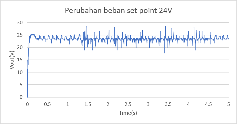
Fig. 20 presents the experimental output-voltage response under load variation at a 24 V set point, showing that the output voltage remains regulated around the reference value despite load changes. Based on dynamic load disturbance testing at a 24 V set point for 5 seconds, the system exhibited adaptive response characteristics. When switched on (0–0.2 seconds), the output voltage (Vout) quickly rises from 0 V to the 24 V target, followed by a small overshoot to 25.2 V (<5%). During operation with a 100Ω load from 0 to 1.35 seconds, the system maintains a stable steady-state phase of 24 V with a regular voltage ripple (<10%). Transitioning the load to 300Ω at intervals of 1.35–4.2 seconds triggers a spike or denser transient noise up to 28 V. However, the control algorithm has been shown to keep the average voltage near the reference value until the test is over.

19. Load change testing at 12V setpoint

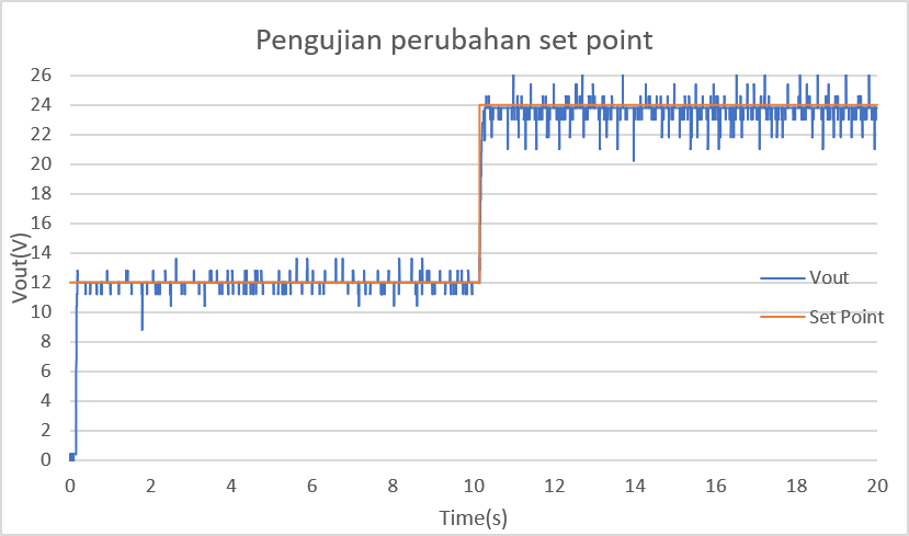
Fig. 21 shows the experimental set-point change test, with the output voltage transitioning from 12 V to 24 V while maintaining regulation around each reference value. A 20-second set-point tracking graph shows the control system's fast, precise signal-tracking capabilities. In the initial phase (0 to 10 seconds), the system operates steadily following the first set-point of 12 V with a voltage ripple of less than 10% that oscillates around the reference value. When the set-point steps to 24 V in the 10th second, the output voltage (Vout) responds quickly (rise time <0.2 seconds) without significant overshoot or undershoot. From the 10th to the 20th second, the system maintains a steady state at 24 V with regular, proportional ripple oscillations (<10%).

20. Load change testing at 24V setpoint

21. Setpoint change testing

1. Comparison of PI-AW and AFPID

1. Load Change in Buck Mode from 100Ω to 300Ω

This test evaluated the output voltage response characteristics of the Non-Inverting Buck-Boost Converter at a set point of 12 V. Test results were compared between the PI Anti-Windup (PI AW) and AFPID methods to assess each controller's ability to reach the reference value and maintain output-voltage stability. The observed parameters included rise time, peak time, overshoot, settling time, steady-state error, and ripple voltage.

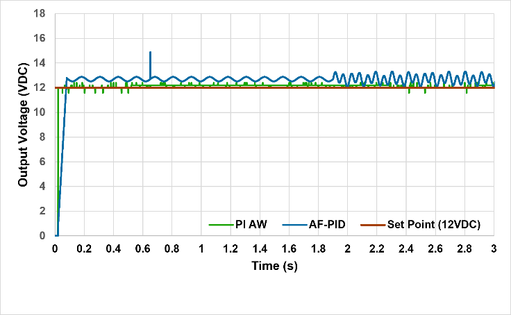
Fig. 22 compares the PI-AW and AF-PID controller responses for a 12 V set point. Both controllers are able to regulate the output voltage close to the reference value, with the PI-AW controller stabilizing at approximately
12.4–12.5 V, while the AFPID controller stabilizes at approximately 12.5–12.7 V. These results are consistent with the performance data presented in Table 12, where the PI-AW controller achieves a rise time of 0.03 s, peak time of 0.04 s, overshoot of 3.3%, settling time of 0.06 s, and steady-state error of 0%. In comparison, the AF-PID controller exhibits a rise time of 0.08 s, peak time of 0.66 s, overshoot of 24.2%, settling time of 3 s, and steady-state error of 5.8%. The ripple voltage is also lower for PI-AW, at 0.15–0.25 , compared with 0.6–1.1  for AF-PID. These results indicate that both controllers regulate the output around the 12 V reference, but their measured transient and steady-state characteristics differ, as summarized in Table 12.

Based on Fig. 22, the two control methods can drive the output voltage to a reference value of 12 V. However, the resulting response characteristics differ significantly. The Anti-Windup PI controller produces a faster response with relatively small overshoot and can achieve tune-like conditions in a short time. In contrast, the AFPID method still exhibits higher overshoot and oscillations after the system reaches steady state, causing the output voltage to fluctuate around the reference value.

22. Load testing output voltage graph 100Ω to 300Ω on buck mode control PI-AW and AFPID

12. Response Parameters Comparison Buck Mode Control PI-AW, and AFPID at 100 Ω to 300 Ω Load

2. Load Change in Boost Mode From 100Ω to 300Ω

This test aims to evaluate the ability of the PI Anti-Windup (PI-AW) controller to maintain the output voltage of the Non-Inverting Buck-Boost Converter with a set point of 24 V, and then compare it with the AFPID method in Fig.23.

Evaluation was carried out based on the characteristics of transient response and the constant condition of the system, including rise time, peak time, overshoot, settling time, steady-state error, and ripple output voltage.

Table 13 shows that the Anti-Windup PI provides better control performance than the AFPID in the 24 V setpoint test. In addition, the Anti-Windup PI output voltage stays close to the reference value with relatively low ripple and oscillation. In contrast, AFPID still shows considerable voltage fluctuations, accompanied by several spikes, after the system reaches a tuned state. This results in lower AFPID voltage-regulation quality than PI Anti-Windup. Thus, the test results show that the PI Anti-Windup controller better maintains output-voltage stability in the Non-Inverting Buck-Boost Converter under both transient and steady-state conditions.

23. Load testing output voltage graph 100Ω to 300Ω on boost mode control PI-AW and AFPID

13. Response Parameters Comparison of PI-AW Control Boost Modes, and AFPID at 100 Ω to 300 Ω Load

4. Conclusion

This research has successfully designed and implemented two voltage control methods, namely Proportional-Integral Anti-Windup (PI-AW) and Adaptive Fuzzy PID (AFPID), on the DC-DC Buck-Boost Non-Inverting converter based on the ESP32 microcontroller. Both methods were tested in simulation using PSIM and in hardware in buck mode (12 V) and boost mode (24 V), with test scenarios including fixed set points, set-point changes, and load changes. The test results showed that both methods maintained the output voltage to follow the reference values in all test scenarios. However, based on transient response parameters and tubular conditions, the Anti-Windup PI provides better performance than the Adaptive Fuzzy PID. In the load change test with a 12 V set point, the Anti-Windup PI also produced a lower overshoot of about 0.03 s, an overshoot of 3.3%, a settling time of about 0.06 s, a steady-state error close to 0%, and a ripple voltage of 0.15–0.25 Vpp.

Meanwhile, at the 24 V set point, the Anti-Windup PI also produced lower overshoot (about 1.3%), with a settling time of about 0.07 s and a ripple voltage of 0.3–0.5 Vpp.  AFPID still shows greater oscillations and voltage spikes under load-change conditions. This performance shows that the Anti-Windup mechanism with the back-calculation method limits integral accumulation when the actuator is saturated, so the transient response becomes faster, overshoot is suppressed, and output-voltage stability is easier to maintain. Thus, under the system specifications and test conditions used in this study, PI Anti-Windup is a more effective control method than Adaptive Fuzzy PID for maintaining output-voltage stability in the DC-DC Buck-Boost Non-Inverting converter.

References

1. K. Salitha, H. A. Vidya, and J. Ramprabhakar, “Advancement of Power Electronic Converter and Control Methods in Microgrid Systems: A Review,” IEEE Access, vol. 14, pp. 4402–4434, 2026, https://doi.org/10.1109/ACCESS.2025.3650614.
2. S. Prasad, K. Ranawat, P. Prabhakaran, and A. Dominic, “A Novel Switched Capacitor-Based Dual-Input Converter for Solar PV and Battery Interface,” IEEE Journal of Emerging and Selected Topics in Power Electronics, vol. 13, no. 6, pp. 6863–6876, 2025, https://doi.org/10.1109/JESTPE.2025.3565215.
3. B. Chandrasekar et al., “Non-Isolated High-Gain Triple Port DC-DC Buck-Boost Converter with Positive Output Voltage for Photovoltaic Applications,” IEEE Access, vol. 8, pp. 113649–113666, 2020, https://doi.org/10.1109/ACCESS.2020.3003192.
4. W. Han, T. Wik, A. Kersten, G. Dong, and C. Zou, “Next-Generation Battery Management Systems: Dynamic Reconfiguration,” IEEE Industrial Electronics Magazine, vol. 14, no. 4, pp. 20–31, 2020, https://doi.org/10.1109/MIE.2020.3002486.
5. X. Weng, Z. Zhao, K. Chen, L. Yuan, and Y. Jiang, “A Nonlinear Control Method for Bumpless Mode Transition in Noninverting Buck-Boost Converter,” IEEE Transactions on Power Electronics, vol. 36, no. 2, pp. 2166–2178, 2021, https://doi.org/10.1109/TPEL.2020.3007600.
6. G. Chen and K. H. Loo, “Voltage Gain-Based Control for Four-Switch Buck-Boost Converter Exhibiting Fast Dynamic Response Over Wide Output Voltage and Load Range,” IEEE Transactions on Power Electronics, vol. 41, no. 7, pp. 12016–12030, 2026, https://doi.org/10.1109/TPEL.2026.3659103.
7. A. C. Handika, S. M. Ilman, F. A. S. Putra, Y. S. Halomoan, G. V. Pratama, and M. N. Ar-Rabbani, “Voltage Control on Non-Inverting Buck-Boost DC-DC Converter with the Digital PI Method,” JTEIN: Jurnal Teknik Elektro Indonesia, vol. 7, no. 1, pp. 13–24, 2026, https://doi.org/10.24036/jtein.v7i1.798.
8. A. Russo, G. P. Incremona, R. Seeber, and A. Ferrara, “Adaptive Bounded Integral Control with Enhanced Anti-Windup Design,” IEEE Control Systems Letters, vol. 7, pp. 1861–1866, 2023, https://doi.org/10.1109/LCSYS.2023.3282378.
9. B. Sarsembayev, K. Suleimenov, and T. D. Do, “High Order Disturbance Observer Based PI-PI Control System with Tracking Anti-Windup Technique for Improvement of Transient Performance of PMSM,” IEEE Access, vol. 9, pp. 66323–66334, 2021, https://doi.org/10.1109/ACCESS.2021.3074661.
10. N. W. Madebo, “Enhancing Intelligent Control Strategies for UAVs: A Comparative Analysis of Fuzzy Logic, Fuzzy PID, and GA-Optimized Fuzzy PID Controllers,” IEEE Access, vol. 13, pp. 16548–16563, 2025, https://doi.org/10.1109/ACCESS.2025.3532743.
11. A. Laib, B. Talbi, A. Krama, and M. Gharib, “Hybrid Interval Type-2 Fuzzy PID+I Controller for a Multi-DOF Oilwell Drill-String System,” IEEE Access, vol. 10, pp. 67262–67275, 2022, https://doi.org/10.1109/ACCESS.2022.3185021.
12. A. Rodriguez-Lorente, A. Barrado, C. Calderon, C. Fernandez, and A. Lazaro, “Non-inverting and Non-isolated Magnetically Coupled Buck-Boost Bidirectional DC-DC Converter,” IEEE Transactions on Power Electronics, vol. 35, no. 11, pp. 11942–11954, 2020, https://doi.org/10.1109/TPEL.2020.2984202.
13. M. A. B. Kumar and V. Krishnasamy, “A Single-Switch Continuous Input Current Buck-Boost Converter With Noninverted Output Voltage,” IEEE Transactions on Power Electronics, vol. 38, no. 2, pp. 2181–2190, 2023, https://doi.org/10.1109/TPEL.2022.3215179.
14. J. Moon et al., “60-V Non-Inverting Four-Mode Buck-Boost Converter with Bootstrap Sharing for Non-Switching Power Transistors,” IEEE Access, vol. 8, pp. 208221–208231, 2020, https://doi.org/10.1109/ACCESS.2020.3038444.
15. M. Martinez-Lopez, M. Cucuzzella, J. M. Guerrero, and J. Moreno-Valenzuela, “Anti-Windup Adaptive PID Control for Trajectory Tracking in Input-Constrained Power Converters,” IEEE Control Systems Letters, vol. 9, pp. 2187–2192, 2025, https://doi.org/10.1109/LCSYS.2025.3597926.
16. H. B. Shin and J. G. Park, “Anti-windup PID controller with integral state predictor for variable-speed motor drives,” IEEE Transactions on Industrial Electronics, vol. 59, no. 3, pp. 1509–1516, 2012, https://doi.org/10.1109/TIE.2011.2163911.
17. A. J. Prado, M. Herrera, X. Dominguez, J. Torres, and O. Camacho, “Integral Windup Resetting Enhancement for Sliding Mode Control of Chemical Processes with Longtime Delay,” Electronics (Switzerland), vol. 11, no. 24, p. 4220, 2022, https://doi.org/10.3390/electronics11244220.
18. M. A. A. Murad and F. Milano, “Modeling and Simulation of PI-Controllers Limiters for the Dynamic Analysis of VSC-Based Devices,” IEEE Transactions on Power Systems, vol. 34, no. 5, pp. 3921–3930, 2019, https://doi.org/10.1109/TPWRS.2019.2911034.
19. Y. J. Lee, A. Khaligh, and A. Emadi, “A compensation technique for smooth transitions in non-inverting buck-boost converter,” in Conference Proceedings - IEEE Applied Power Electronics Conference and Exposition - APEC, Washington, DC, USA, 2009, pp. 608–614, https://doi.org/10.1109/APEC.2009.4802721.
20. R. G. Kanojiya and P. M. Meshram, “Optimal tuning of PI controller for speed control of DC motor drive using particle swarm optimization,” in 2012 International Conference on Advances in Power Conversion and Energy Technologies, APCET 2012, Mylavaram, India, pp. 1–6, 2012, https://doi.org/10.1109/APCET.2012.6302000.
21. M. H. Azam, M. H. Hasan, S. Hassan, and S. J. Abdulkadir, “A Novel Approach to Generate Type-1 Fuzzy Triangular and Trapezoidal Membership Functions to Improve the Classification Accuracy,” Symmetry, vol. 13, no. 10, p. 1932, Oct. 2021, https://doi.org/10.3390/sym13101932.
22. Z. J. Zhou, G. Y. Hu, C. H. Hu, C. L. Wen, and L. L. Chang, “A Survey of Belief Rule-Base Expert System,” IEEE Transactions on Systems, Man, and Cybernetics: Systems, vol. 51, no. 8, pp. 4944–4958, 2021, https://doi.org/10.1109/TSMC.2019.2944893.
23. Sunardi, A. Yudhana, and Furizal, “Tsukamoto Fuzzy Inference System on Internet of Things-Based for Room Temperature and Humidity Control,” IEEE Access, vol. 11, pp. 6209–6227, 2023, https://doi.org/10.1109/ACCESS.2023.3236183.
24. M. Whitby, L. Cardelli, M. Kwiatkowska, L. Laurenti, M. Tribastone, and M. Tschaikowski, “PID Control of Biochemical Reaction Networks,” IEEE Transactions on Automatic Control, vol. 67, no. 2, pp. 1023–1030, 2022, https://doi.org/10.1109/TAC.2021.3062544.
25. D. Wu, R. Peng, and J. M. Mendel, “Type-1 and Interval Type-2 Fuzzy Systems [AI- eXplained],” IEEE Computational Intelligence Magazine, vol. 18, no. 1, pp. 81–83, 2023, https://doi.org/10.1109/MCI.2022.3223496.
26. S. H. Khairuddin, M. H. Hasan, M. A. Hashmani, and M. H. Azam, “Generating clustering-based interval fuzzy type-2 triangular and trapezoidal membership functions: A structured literature review,” Symmetry, vol. 13, no. 2, pp. 1–25, 2021, https://doi.org/10.3390/sym13020239.
27. Q. A. Tarbosh et al., “Review and Investigation of Simplified Rules Fuzzy Logic Speed Controller of High Performance Induction Motor Drives,” IEEE Access, vol. 8, pp. 49377–49394, 2020, https://doi.org/10.1109/ACCESS.2020.2977115.
28. N. G and K. J, “Performance comparison between PID and Fuzzy logic controllers for the hardware implementation of traditional high voltage DC-DC boost converter,” Heliyon, vol. 10, no. 17, p. e36750, Sep. 2024, https://doi.org/10.1016/j.heliyon.2024.e36750.
29. A. H. A. Adam et al., “Power Decoupling Enhancement of a Triple Active Bridge Converter with Feedforward Compensation Based on Model Predictive Control and Fuzzy Logic Controller in DC Microgrid Systems,” IEEE Access, vol. 12, pp. 140310–140328, 2024, https://doi.org/10.1109/ACCESS.2024.3469815.
30. J. Pakdeeto, S. Wansungnoen, K. Areerak, and K. Areerak, “Optimal Speed Controller Design of Commercial BLDC Motor by Adaptive Tabu Search Algorithm,” IEEE Access, vol. 11, pp. 79710–79720, 2023, https://doi.org/10.1109/ACCESS.2023.3300233.
31. M. A. George, D. V. Kamat, and C. P. Kurian, “Electronically Tunable ACO Based Fuzzy FOPID Controller for Effective Speed Control of Electric Vehicle,” IEEE Access, vol. 9, pp. 73392–73412, 2021, https://doi.org/10.1109/ACCESS.2021.3080086.
32. J. Sarathi and D. Rama Prabha, “An Effective ANFIS Approach for Interconnected DFIG-Based Wind Energy System With Model-In-Loop Validation,” IEEE Access, vol. 13, pp. 77147–77164, 2025, https://doi.org/10.1109/ACCESS.2025.3565073.