Journal of Fuzzy Systems and Control, Vol. 1, No 3, 2023 |
GWO-PID of Two-Phase Hybrid Stepping Motor for Robotic Grinding Force
Fatin Nabeel Abdullah 1, Ghada Adel Aziz 2 Salam Waley Shneen Jaeb 3,*
1,2,3 University of Technology - Iraq, Baghdad, Iraq
Email: 1 50060@uotechnology.edu.iq, 2 50070@uotechnology.edu.iq, 3 salam.w.shneen@uotechnology.edu.iq
*Corresponding Author
Abstract—The use of the computer program MATLAB is prominent in many studies that simulate many industrial systems. The current simulation aims to build a suitable simulation model representing the Two-phase Hybrid Stepping Motor (2Ph-HSM). This type of motor is employed in a specific application to produce a force called automatic grinding force. To control the force, motor speed, and location, we need to add control systems, so two methods have been proposed, one of which is traditional, namely proportional, integral, and derivative (PID) control and the other is intelligent, called Gray Wolf Optimization (GWO). The current work also aims to use traditional control algorithms and advanced optimization algorithms that were chosen for their ease of control and possibility of use in many industrial applications. By setting appropriate specifications for the simulation model and after conducting prescribed tests that simulate different applications of the motor’s work within electrical systems, the results demonstrated good motor performance, better response, and high accuracy, in addition to speed. The goal is to design and tune a proportional, integral, and derivative (PID) controller by gray wolf optimization (GWO) using the transfer function (TF) of a 2Ph-HSM. To adjust the parameters of conventional controllers using advanced optimization, a suitable mechanism and technique were selected from advanced optimization techniques, where the gray wolf technique algorithm was chosen as an optimization technique and Integrated Time Absolute Error (ITAE) to adjust the parameters of conventional PID controller.
Keywords— GWO-PID; PID; RGS; 2Ph-HSM
Previous studies confirmed the possibility of using computer programs, including the MATLAB engineering program, to simulate systems that focus on operating electric motors in various fields. Previous studies have also confirmed the possibility of representing electric motors with mathematical models and block diagrams [1]-[5]. The conversion function of the system can be calculated according to the appropriate specifications. The 2Ph-HSM motor is one of the motors that has gained a great deal of importance in industrial applications, including moving and rotating a robot arm in the grinding process of curved surfaces such as a fan. The ship is the subject of current simulations [6]-[10].
Electric motors need control units to improve their performance. Among the commonly used control units that have proven their efficiency with linear systems is the traditional controller [11]-[15]. While nonlinear systems need expert units such as neural networks and fuzzy logic or smart ones such as the optimal advance of a genetic algorithm or types. The work environment is considered to be on a turbine blade or a marine fan that needs an environment suitable for constant force. The grinding process bends with the change of time. The workpiece bends on the work piece. We need to provide the required natural path for the grinding process accurately because of changing its dimensions during the grinding process and changing the dimensions as a result of the erosion of the piece by the impact of the grinding process [16]-[19].
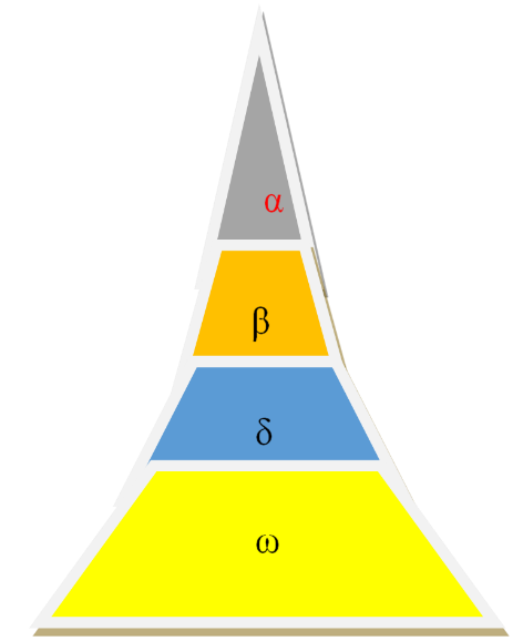
The hierarchical wolf algorithm is one of the most important algorithms that previous experiments have demonstrated the possibility of using to improve the performance of linear and nonlinear systems. Among the categories that it includes is the leader and it is called alpha (a), which is considered the highest in the hierarchy or from the first level. The leader category is the one that cares and is able to make decisions, including choosing the spatial environment for hunting and the place to live. It does not matter if the leader is female, male, or both. Another category is beta (ꞵ), which is from the second level of the hierarchy, and this category assists the first category in making some decisions. There is also a third category, Delta (δ), and it is the lowest level in terms of hierarchy, and it is the category that is subject to orders. All categories are in the form of groups, and each has a role to play or what is called a scapegoat [20]-[24]. Finally, the Omega category (ꙍ), which is the lowest category of the pyramid, or the fourth rank is called the category of sheiks, and its function is detection and guarding. All classes in the algorithm hierarchy can be represented by a flowchart of the wolves’ algorithm as in the Fig. 1. Whereas Fig. 2 show the flow process of the method.
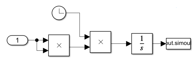
Performance indicators of the error in the system are the problem and its solution is to get rid of it completely or reduce it to the lowest possible level, thus obtaining an effective system design within the required outputs. The amount of error is taken and treated with one of the techniques of system performance indicators such as IAE, which means absolute integration of error [25]-[29]. There are other types that will be mentioned and represented in the equations (1-4) and Fig. 3, Fig. 4, Fig. 5, Fig. 6.
| (1) | |
| (2) | |
| (3) | |
| (4) |
To obtain an effective and appropriate system response, an objective function of the type ITAE was chosen. It means the integration of the absolute error multiplied by time. It is based on the measurement of the error value during operation e(t) and is calculated from the difference between the actual speed (feedback) and the reference (required). It can be mathematically represented by an equation and as a model [30]-[34].
After representing the model mathematically and arriving at a transfer function model that fits its specifications, the proposed tests were performed. The simulation results showed the possibility of representing and simulating the system in addition to the possibility of improving performance for the various proposed cases. In this simulation, we propose to test the possibility of representing the robotic arm, which is driven using an electric motor, to perform the milling process of a curved surface of the ship's hull from under the water, which requires a balanced effort and force to perform the work with high accuracy and proficiency. Therefore, this requires that all operating conditions be considered according to a suitable controller's business strategy and algorithm for its real-time operation [35]-[39].
The model can be represented mathematically and appropriate tests can be performed to simulate real-time operation. Three tests were developed for the purpose of comparison and to determine the importance of each condition and the negatives and positives through the simulation results of response speed, ascent, overtaking, stability, transient condition, and all associated working conditions. Improving work performance by adopting intelligent control systems that are compatible with the non-linear system, since the traditional control unit is only suitable for linear systems [40]-[44].
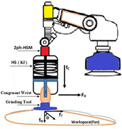
The grinding process is a mechanical process provided by the electric motor. The grinding process takes place as a result of the presence of materials to be removed from the surfaces of the required workpieces. The 2ph-HSM motor is used in the milling process as a result of its suitable torque as well as being suitable in terms of noise, vibration, and cost. The milling machine can be seen in Fig. 7, where there are clear forces for the milling process, normal, and tangential which are symbolized by fN, fT, and Fd. Fig. 8 represents the scheme of the system, which can be mathematically represented by the equations (5-8) [45]-[50].
After examining the components of the system and representing them mathematically, the next step is to build the simulation model in successive steps. Where: Tangential force is fT, elastic modulus of a Helix Spring is Kf, smallest displacement to compress the Helix Spring is ds, greatest displacement is dg, precise displacement is dp.
| (5) | |
| (6) | |
| (7) | |
| (8) |
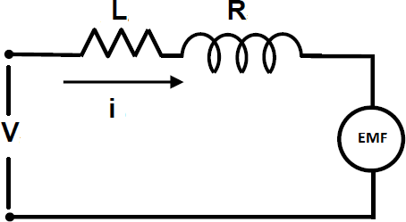
The simulation model can be represented by an equivalent circuit and the appropriate transfer function. It represents the electrical circuit of the motor as in Fig. 9 and the transfer function is in (9).
| (9) |
| |
| |
|
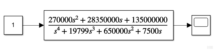
When the system specifications are known, the required transfer function for the simulation model can be written. The system specifications and the transfer function are as follows: Resistance R = 1.3Ω, Inductance L= 4.5mH, Coefficient of Viscous Friction B = 0 N∙m∙s/rad, Inertia Constant J = 270 kg∙m, β = 1, KDv = 115, Kpv = 550, KIi = 550, KIv = 0, ke = 0.25 N∙m/A, KH = 10, KPi = 6 and N = 180. Transfer function (TF) will be (10).
| (10) |
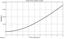
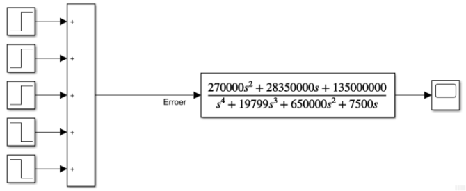
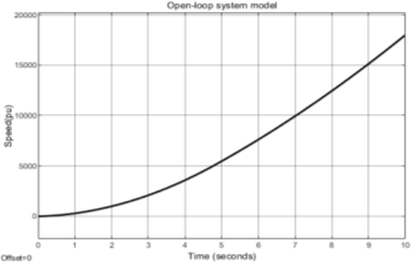
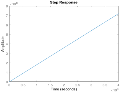
The behavior of the open-loop system can be studied in both linear and nonlinear systems using model and simulation results. For example, the reference value of the system is speed, and when the system operates with a fixed reference value of speed, this type is considered a linear system that can represent the simulation model as in Fig. 10 (a). The behavior of the system can be known through the simulation results as in Fig. 10 (b) while the non-linear system, which is when the system operates with a variable speed reference value, can represent the simulation model as in Fig. 11 (a) and the behavior of the system can be known through the simulation results as in Fig. 11 (b). From the figure, we notice the instability of the system is clear. This requires finding a solution for the stability of the system. It is suggested to build a closed-loop system and conduct a test to know the behavior of the system.
a. Simulation model
b. Simulation result
a. Simulation model
b. Simulation result
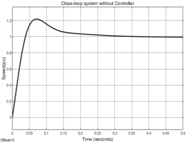
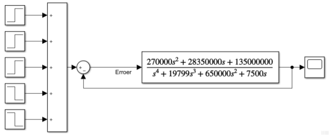
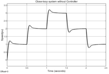
The behavior of the closed-loop system without a controller can be studied in both linear and nonlinear systems using model and simulation results. For example, the reference value of the system is speed, and when the system operates with a fixed reference value of speed, this type is considered a linear system that can represent the simulation model as in Fig. 12 (a). The behavior of the system can be known through the simulation results as in Fig. 12 (b), while the non-linear system, which is when the system operates with a variable speed reference value, can represent the simulation model as in Fig. 13 (a) and the behavior of the system can be known through the simulation results as in Fig. 13 (b).
a. simulation model without controller
b. Simulation result without controller
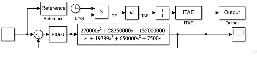
The simulation model in Fig. 12 shows the conversion function with the reference signal and the oscilloscope for the (actual) output signal. We also note the presence of feedback, as well as a comparator between the reference and actual value, and the output of the comparator represents the error value. Fig. 13 represents the output of the oscilloscope and represents the closed-loop system behavior.
From the figure, we notice the transient state and the stable state by exceeding the output from the established limit, and then it returns to the required value. This requires finding a solution for the stability of the system while reducing the rate of overshot and speed of performance. It is suggested to build a closed loop system with a conventional control unit and conduct the test to know the behavior of the system.
a. simulation model without controller
b. Simulation result without controller
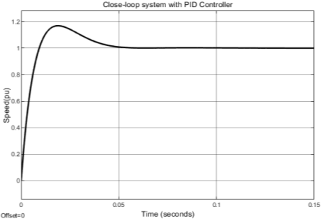
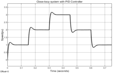
The behavior of the closed-loop system with PID controller can be studied in both linear and nonlinear systems using model and simulation results. For example, the reference value of the system is speed, and when the system operates with a fixed reference value of speed, this type is considered a linear system that can represent the simulation model as in Fig. 14 (a). The behavior of the system can be known through the simulation results as in Fig. 14 (b), while the non-linear system, which is when the system operates with a variable speed reference value, can represent the simulation model as in Fig. 15 (a) and the behavior of the system can be known through the simulation results as in Fig. 15 (b).
a. simulation model with PID controller
b. simulation results with PID controller
a. simulation model with PID controller
b. Simulation results with PID controller
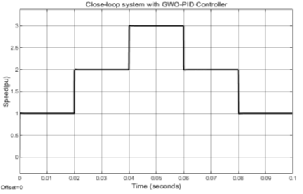
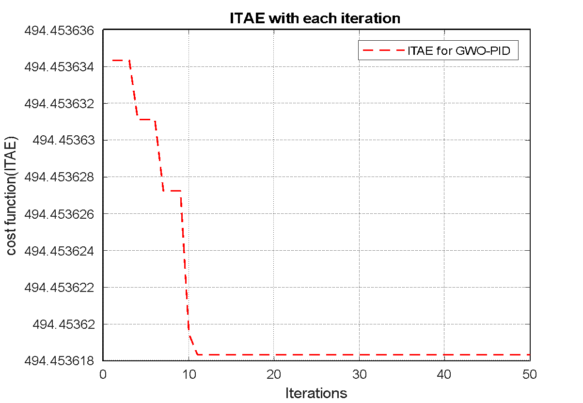
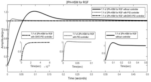
The behavior of the closed-loop system with GWO-PID controller can be studied in both linear and nonlinear systems using model and simulation results. For example, the reference value of the system is speed, and when the system operates with a constant reference value of speed, this type is considered a linear system that can represent the simulation model as in Fig. 16 (a). The behavior of the system can be known through the simulation results as in Fig. 16 (b), while the non-linear system, which is when the system operates with a variable speed reference value, can represent the simulation model as in Fig. 17 (a) and the behavior of the system can be known through the simulation results as in Fig. 17 (b). Performance using the ITAE objective function with GWO-PID controller is shown in Fig. 18. The results can be appended in one form to show the difference between the different methods and to identify the best among them, as in Fig. 19.
a. Simulation model with GWO-PID controller
b. Simulation results with GWO-PID controller
a. Simulation model with GWO-PID controller
b. Simulation results with GWO-PID controller
To discuss the simulation results, we need to describe the behavior of the system for the proposed cases and adopt the comparison between the different tests. The measurement criteria are time, such as the rise time, the settling time, and the average rate of deviations from the desired goal. The fastest method is considered the best, and the least deviation rate characterizes the best method. The fastest way is by using the gray wolf algorithm and the lowest bypass rate was by the wolf algorithm.
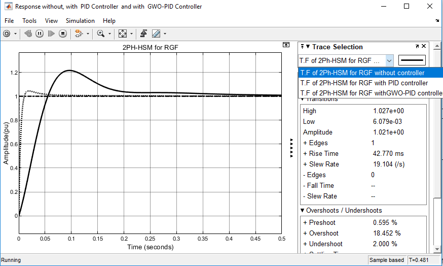
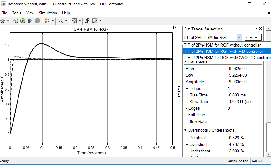
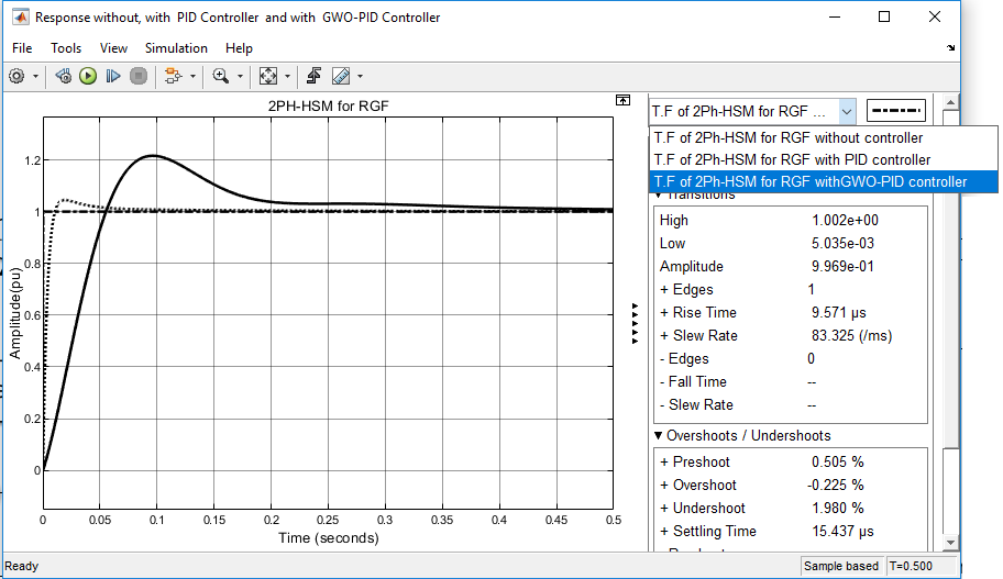
In the simulation results section, there are three parts, The first part simulation model, under title modeling without a controller which means a close loop at the linear system, and the result of this model is shown in Fig. 20. Fig. 20 shows the rise time equal 42.7 ms, overshoot of 18.452%, and undershoot 2%. The second part, the simulation model under title modeling with PID controller at the close loop at liner system and the result of this model is shown in Fig. 21. Fig. 21 shows the rise time equal 6.603ms, overshoot amplitude equal 4.737% and undershoot 2%. Finally, part, simulation model, under title modeling with GWO-PID controller means a close loop at the liner system, and the result of this model is shown in Fig. 22. Fig. 22 shows the rise time equal to 9.571ms, overshoot of -0.225%, undershoot of 1.980%, and settling time equal to 15.437 ms.
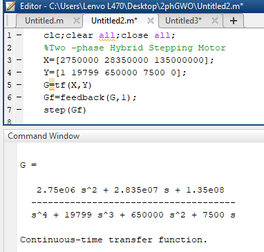
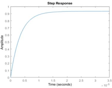
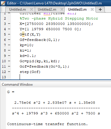
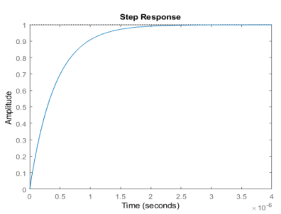
Another method of simulation can be presented by writing code that represents the system in the form of m-files, as in the forms of simulation models and simulation results in the following forms: First, open loop system, the modeling m-file as shown in Fig. 23 (a) and the simulation result as shown in Fig. 23 (b). Second, the close loop system without a controller, the modeling m-file as shown in Fig. 24 (a), and the simulation result as shown in Fig. 24 (b). Third, the close loop system with PID controller, the modeling m-file as shown in Fig. 25 (a), and the simulation result as shown in Fig. 25 (b). Fourth, the close loop system with GWO-PID controller, the modeling m-file as shown in Fig. 26 (a), and the simulation result as shown in Fig. 26 (b).
a. The modeling by m-file
b. The results by m-file
a. The modeling by m-file
b. The results by m-file
a. The modeling by m-file
b. The results by m-file
a. The modeling by m-file
b. The results by m-file
Simulation and engine model building were performed using MATLAB (SIMULINK) software. Specifications were chosen to fit the proposed application to run a motor in a robotic system for surface grinding process, such as a turbine fan or a steamer. The effectiveness of the model and the validity of the system were also verified. The possibility of improving the performance of the motor with different working conditions similar to real-time operation was verified. The aim of the research is to simulate a working system of a robot that is managed and moved by the proposed electric motor of the two-phase hybrid stepper motor by adopting the use of the computer and building the model from the MATLAB program package to perform the grinding process and control the force as a result of the surface difference during the grinding process. The advantage and clear superiority of the smart system over the traditional one, and the control using a traditional unit is also effective in the process of improving performance with the system.
Fatin Nabeel Abdullah, GWO-PID of Two-Phase Hybrid Stepping Motor for Robotic Grinding Force